8 ways to bring powerful new comparisons to viz audiences with Tableau set actions


Interactivity is a core component of rich analytical systems. It helps answer deeper questions, solve more end user tasks, and create improved user experiences. More expressive interactivity means you can provide richer content for audiences such as clients and stakeholders. Playful experiences drive curiosity and engagement, two crucial ingredients to improving data literacy throughout the world.
Until now, Tableau’s interactivity has centered on specific action types, such as filtering and highlighting. While authors can control the source and targets of these actions, their behaviour is fixed. Highlight actions always highlight, but what if you wanted to colour your selection? Filters always filter all fields, but what if you wanted to filter a single axis to compare it to the total?
New interaction behaviours with set actions
Sets are powerful. They allow user selections to be used anywhere in a visualization and in calculations. Sets can colour, group, and filter an axis in a viz or a term in a calculation. They can also conditionally aggregate, combine fields, hide data that is used in a table calculation, and filter on a related field—and that’s just the start.
The new set action feature in Tableau 2018.3 means that a selection of data points in a visualization can be stored in a set. Set actions are much more than a new type of action; they extend Tableau's interactivity to support custom user-defined behaviour.
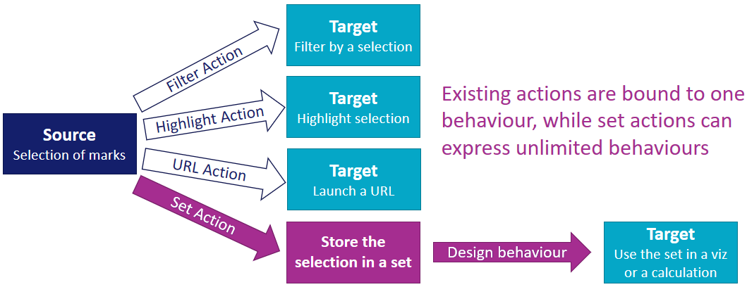
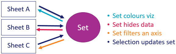
A set can apply different behaviours to various target sheets. For example, the same set could colour viz A, hide data in viz B, and filter an axis in viz C. Now with set actions, a user selection in any of the sheets can update the set, thereby modifying all target sheets in a single coordinated selection. Coordinating multiple actions through a single selection dramatically increases the breadth and depth of scenarios that can be addressed for end users though interactive analytic applications.
While this post focuses specifically on comparative analytics, the second post introduces many new interactive analytics techniques expressed with set actions.
Learning Objectives
Set actions connect two existing features, offering a wealth of opportunity to create new compositions from existing concepts. In this post, we'll explore examples of part-to-whole analysis, part-to-part analysis, and difference from a selection. While set actions have made all of the scenarios presented here possible, the goal of the examples is to demonstrate end-to-end user flows. Some of the things you can expect to learn from the following examples:
- New ways to provide rich comparative context that improves the interpretation and communication of data.
- How data structure impacts calculations, and when to use table calculations versus level of detail expressions.
- Using interactivity to represent multiple concepts at once, such as change over time, relative difference, and part to whole analysis.
You may follow the video tutorials using the data sources here, which can be accessed using a trial of Tableau Desktop.
Part-to-whole analysis
Have you ever wanted to analyse how a selection contributes to the total? Sometimes you may want to calculate its contribution as a percent of total. Alternatively, you may want to see its magnitude against the total. In other cases, you may wish to calculate differences between your selection and the total. This section will demonstrate all of these concepts. The first 3 examples incrementally build on one another, so you may want to watch the video demos in order!
Example 1: Selection as a percent of total
- Concept: While filters only keep data in a selection, sets split data into two groups—in or out of the selection. Retaining all the data means that you can easily compute a selection's contribution to the total.
- Data source: Market Value of Players and Teams in the 2018 World Cup
- Scenario: What is the market value for a selected team, group, or region as a percent of the total market value of players in the 2018 World Cup? How does that compare to the percent of teams represented by the selection?
- Interpretation: When Europe is selected, you can see that it represents 66% of the market value but only 44% of the teams.
- Noteworthy: This is a Pareto principle exposed through interaction. Interactivity is a way to expose statistical concepts in a simple way!

Example 2: Proportional brushing
- Concept: Proportional Brushing is an interactive analytics technique that displays the magnitude of a selection relative to the total magnitude.
- Scenario: Which player positions have the highest market value? For a selection of teams, what proportion do they contribute to the overall market value per position?
- Interpretation: When the proportion per position is higher than the percent of teams selected, this means that the selected teams have more valuable players than in the world in general. When the proportion per position differs from the overall percent of market value represented by the selected teams, this indicates the relative strength or weakness of a position within the selection.
- Noteworthy: While filters report on what the numbers are, sets help interpret and explain the results.

Example 3: Difference in overall rank and rank across a selection
- Concept: Sets enable targeted filtering. You can use sets to apply filters to a single axis or a subset of fields in a viz, while filters apply to all fields in a target viz.
- Scenario: In the previous example, changing the sort between overall and selection causes the positions to jump. This requires a user to toggle back and forth to compare overall position rankings to rankings across a selection of teams. Wouldn't it be nice to compare ranks across all positions in a single view? This is achieved in the next evolution of part-to-whole analysis!
- Interpretation: The bars on the left rank positions by total market value, while the bars on the right rank positions within the selected country. The connecting lines are horizontal when the selected team's rank matches the overall rank, such as for England’s top two positions. Red downward lines indicate that the selected team has a lower rank than the overall market for the position, while blue upward lines indicate the reverse.
- Noteworthy: In the crisscross view, the left axis never changes. Sets mean that the filters are only targeting the right axis and the colour!

Part-to-part analysis
In relational data structures, it is easy to perform calculations across columns, such as sales and profit. It is much less trivial to calculate across rows within a single column, such as sales in Europe versus sales in America, or sales in 2017 vs sales in 2018. Set actions have made comparisons across rows dynamic, interactive, and simple!
Example 4: Benchmarking
- Concept: Comparing a measure across two selected subsets of data requires new fields to be generated on the fly. The measure and dimension columns must be dynamically transformed into "Measure for Subset 1" and "Measure for Subset 2". This can be achieved through set actions, because sets are like filters for individual measures.
- Data source: Market Value of Players and Teams in the 2018 World Cup
- Scenario: What is the difference in average player market value between team A and team B? How do the two teams compare across positions? Alternatively, how do the top two European countries compare to the top two South American countries? Or how does the host country, Russia, compare to the rest of the world?
- Interpretation: The vertical axis displays average player market value across the teams selected in orange, while the horizontal axis displays average player market value across the teams selected in blue. Each point on the scatterplot represents a player position. Orange dots means that players in the orange countries have a higher average market value, while blue dots mean that players in the blue countries have a higher average market value.
- Noteworthy: Previously parameters were the only way to achieve this type of benchmarking analysis, however sets are preferable because:
- They enable multi-selection
- They are dynamically linked to the country field
- Their values are set through direct interaction with a visualisation instead of a list
- Their selection domain updates in response to filters, displaying relevant values (for example if applying a filter on region)

Example 5: Range comparisons
Concept: Change over time is one of the most common types of comparative analysis, where flexible selection of the start and end periods is available to viz consumers.
- Data source: Normalized London House Price Data (1995-2018)
- Scenario: Given two selected time periods, what is the growth rate from one period to the next? How does the growth rate compare across different districts?
- Interpretation: The time series view serves as a visual calculator demonstrating how the growth rate is computed. The blue and grey ranges are highlighted in corresponding colours on the time series, and the horizontal lines display the averages across each time range. Note that the summary difference is always equal to the difference between the reference lines!
- Noteworthy: The difference calculation is identical to #4, even though this looks and sounds like a very different scenario. Few concepts are required for wide application!

Difference from a selection
Example 6: Difference from summary average across a selection
- Concept: While filters apply to all fields in the view, the scope of sets can be controlled to apply to a single term in a calculation.
- Data source: Market Value of Players and Teams in the 2018 World Cup
- Scenario: For each team, what is the difference from the average market value across a selection of teams?
- Interpretation: This viz displays market value by team in the 2018 World cup, vs the average across teams. As a user interacts with the visualization by selecting a country, a group, a region, or an arbitrary selection of countries (such as Spanish speaking countries), the average re-computes across the selection.
- Noteworthy: The set is only filtering the average calculation, while a filter would remove all countries from the viz that are not in the selection.

Example 7: Difference from underlying average across a selection
- Concept: While the prior example computes the average across the selected bars, some cases require computing the average across the underlying data of a selection.
- Data source: Normalised London House Price Data (1995-2018)
- Scenario: When comparing the average house price within each postcode to the average across a selection, the comparative average should be computed on the underlying data. This ensures that every property has an equal weighting towards the average. Computing the average across summary data would weight properties inversely to the density of their postcode.
- Interpretation: The number displayed in the upper right viz is the average house price across the selected postcodes. The colour on the map displays the percent difference of each postcode from that number, where orange means more expensive and blue means less expensive.
- Noteworthy: This viz previews dynamic grouping, as the legend highlighting current selections creates a new geographic grouping in response to selection. Dynamic grouping will be demonstrated in much more detail in part 2 of this series!

Example 8: Difference in change between a selection and the total
- Concepts: This example brings together 3 concepts from earlier scenarios - part to whole analysis, change over time, and difference from a selection.
- Data Source: 2017-2018 Stock Ticker Data
- Scenario: Analyzing a single stock in isolation could lead one to conclude that increases and decreases can be attributed to the specific stock; however it may be that the overall market is moving in a certain direction. To account for this, you may wish to compare the change in price for a selected stock or portfolio of stocks to the change in the market in general.
- Interpretation: Comparing the skew of distributions showing how often the stock of interest increases more or less than other stocks highlights its relative performance. Green skewed to the right means the selection is outperforming the market, while red skewed to the left means the market outperforms the selection.
- Noteworthy: Daily change is pre-computed in the data because it's a calculation across rows that does not need to re-compute as selections are made. Daily change for the selection is a level of detail expression because LoDs can propogate a value across rows. The difference in daily change between each stock and the selection is a row level calculation (that references the LoD) because it must be computed for every day and every stock, which is the granularity of the data source. A final level of detail expression per stock and per bin aggregates the number of days each stock increases or decreases more than the selection. This is the horizontal axis in the histogram.

Set actions make comparative analytics more powerful and flexible
Comparative analytics are more powerful and flexible now that sets are accessible to end users. Instead of using parameters for many types of interactive comparisons, you can now use sets to enable multi-selection and direct interaction with a viz instead of a list. Moreover, sets are live linked to your data, and you can express some comparisons simply through dragging and dropping!
The next post introduces 8 new techniques expressed with set actions. In particular, filtering on relationship, sorting and aligning on a selection, applying OR conditions across filters, dynamic grouping, and controlling the order of operations. Check it out!
Related stories
VizQL Data Service from Tableau: Use Your Data, Your Way
 8 August, 2024

When and How to Use Multi-fact Relationships in Tableau
 1 August, 2024

Top data books of 2021
 12 December, 2021