How to pair Tableau and Python for prescriptive analytics with TabPy


A version of this blog post originally appeared on Medium.
TabPy is a Python package that allows you to execute Python code on the fly and display results in Tableau visualisations, so you can quickly deploy advanced analytics applications. The split approach granted by TabPy allows for the best of two worlds – class-leading data visualisation capabilities, backed by powerful data science algorithms. One huge benefit of surfacing Python algorithms in Tableau is that users can tune parameters and evaluate their impact on the analysis in real time as the dashboard updates.
To make this possible, TabPy mainly takes an input/output approach where the data is aggregated according to the current visualisation and tuning parameters are both transferred to Python. The data is processed and an output is sent back to Tableau to update the current visualisation. But let’s say you need the full underlying data set for a calculation, but your dashboard is surfacing an aggregate measure, or you want to show multiple levels of aggregation at the same time. Moreover, you may want to leverage multiple data sources in a single calculation without harming the responsiveness of your dashboard.
In this post, I’ll walk you through an approach that helps you unleash the full power of TabPy for the following scenarios:
- Real-time interaction: You want to have a real-time user interface, minimising the processing time and delay between a parameter change and updated visualisation.
- Multiple levels of aggregation: You want to show (several different) aggregation levels on the same Tableau dashboards, but you need to perform all the calculations using the finest and most granular level, containing all information.
- Various data sources: The back-end calculation is relying on more than a single data source and/or database
- Data transferred between Tableau and Python: Need significant amount of data for each optimisation step, so a lot of data must be transferred between Tableau and the Python back end.
A novel TabPy approach for prescriptive analytics: Step-by-step instructions
To implement TabPy, assuming that both Python and TabPy are already installed, you need to run three steps:
- Prepare a draft Tableau dashboard
- Create calculation routines back end in Python
- Design the Tableau frontend leveraging it
To walk you through the three steps, I designed a use case around complexity reduction through product portfolio optimisation.
The use case: Complexity reduction
The subject of the optimisation is a B2B retailer that experienced growth mainly through mergers and acquisitions (M&As). Because of this inorganic growth, the retailer faces a great deal of complexity, operating on several markets and having a portfolio composed of a thousand SKUs (stock-keeping units) that are divided into several categories and subcategories. To further complicate matters, the SKUs are built in different plants.
The company’s senior management wants to increase margins by removing the least profitable SKUs, but is willing to continue selling lower performers to maintain a certain market share. They are also willing to keep the manufacturing plants running above a target asset utilisation, knowing that to decrease utilisation too far would negatively impact the fixed costs base of each plant.
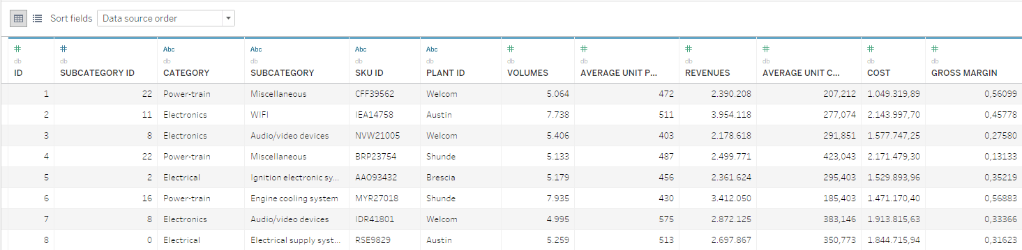
The data available in this example consists of a SKU-level database in which yearly volumes, costs and revenues are reported. The SKUs are organised into Category and Subcategory hierarchical levels.
From a mathematical perspective, the task product portfolio optimisation management faces is fairly straightforward. However, the optimisation must also consider all the strategic nuances and include the participation of a wide range of stakeholders who have access to the information and tools needed to make informed decisions.
All of these requirements are solved by the TabPy approach described below.
1. Prepare a draft Tableau dashboard
First, it is important to align on the problem that needs to be solved. In this example, the simple optimisation algorithm will remove SKUs according to their gross margin, evaluated at the SKU level.
-
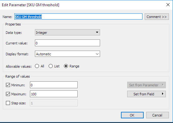
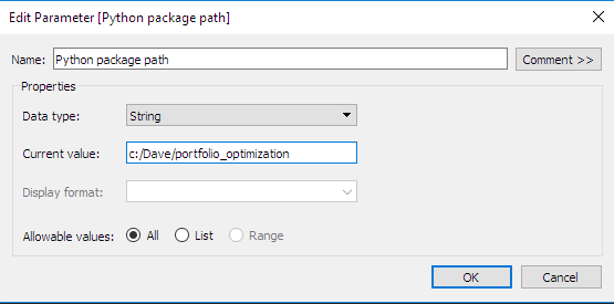
Define the interactive parameters in Tableau: Notice that we’ve defined a second convenience parameter. This is the directory where the Python package with the optimisation routines will be stored. This type of parameter is very useful in defining the custom calculations, as we will see in the next section.
- Define the views/levels of aggregation: Here we define two aggregation levels: an SKU level and a subcategory level. The definition of aggregation levels is key as it dictates the Python back-end functions’ signatures. One specific function must be defined per each calculation and aggregation level. For each aggregation level, the following parameters must be defined: optimised margins, optimised revenues and optimised volumes.
-
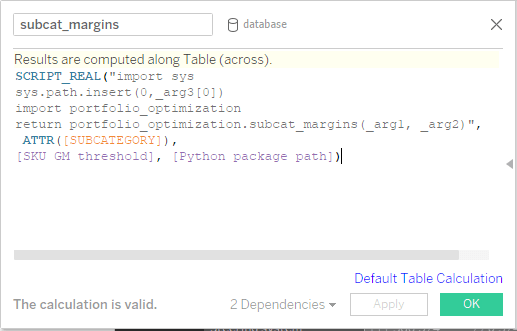
Define calculation hooks (callbacks) in Tableau: Having defined input parameters, aggregation levels and required output calculations, it is possible to define custom calculations. For convenience all the optimisation routines have been structured in a portfolio_optimisation Python package, where we defined functions to return the selected quantities for the specific aggregation levels. It’s worth noticing that the parameter defined earlier – the Python package path – is passed to the function and used in the script to signal where the portfolio optimisation package is stored. Furthermore, the current aggregation level indexer (e.g. for the subcategory aggregation level, the subcategory itself) is always passed to the Python back end to ensure that results will be returned in the proper order. The input parameter, SKU GM threshold, is passed as well.
2. Create calculation routines back end in Python
The Python back end is divided in two function classes, grouped according to their execution context: Functions executed once and those repeated multiple times. In the first class are database extraction and transform and load operations, for example. Such functions are called ‘one-time-operations’. Opposite are the functions that are repeated multiple times, like all the Tableau callbacks:
- One-time operations: In this example, the database is loaded only once, when the script is executed the first time. The database is then made available to all the other functions storing it into a global variable. To detect whether the database is already loaded or not, Python checks the local name space for an existing copy of it. Without this precaution, the database would be loaded any time a calculation is requested by Tableau, negatively impacting execution speed.
- Tableau callbacks: Every hook previously defined must have a function serving it. This is obtained, in our case, providing separated calculations for revenues, volumes and margins, and using the indexer passed as the function’s input, to index the Pandas groupby function that is then used to aggregate optimisation results. It is worth noticing that, to improve the execution speed, callbacks implement a parameter change detector. A new optimisation is spawned only if the parameter is changed and its result will be available to all the callbacks leveraging a global variable. The detection of parameter change is implemented through a persistent variable used to store the value of it at the previous execution. This approach ensures the use of the minimum amount of expensive operations, improving execution speed.
3. Design the Tableau front end
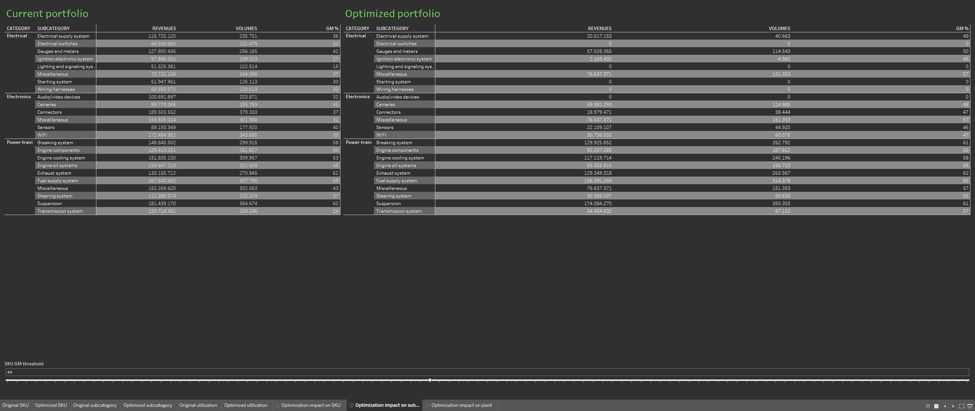
By this step, we've defined all the fundamental bricks, including aggregation levels, parameters to be tuned, and output columns returned by the calculation back end.
To make the optimisation easier to discuss, define two separate worksheets, showing the portfolio before and after the optimisation process. Show the two worksheets side by side.
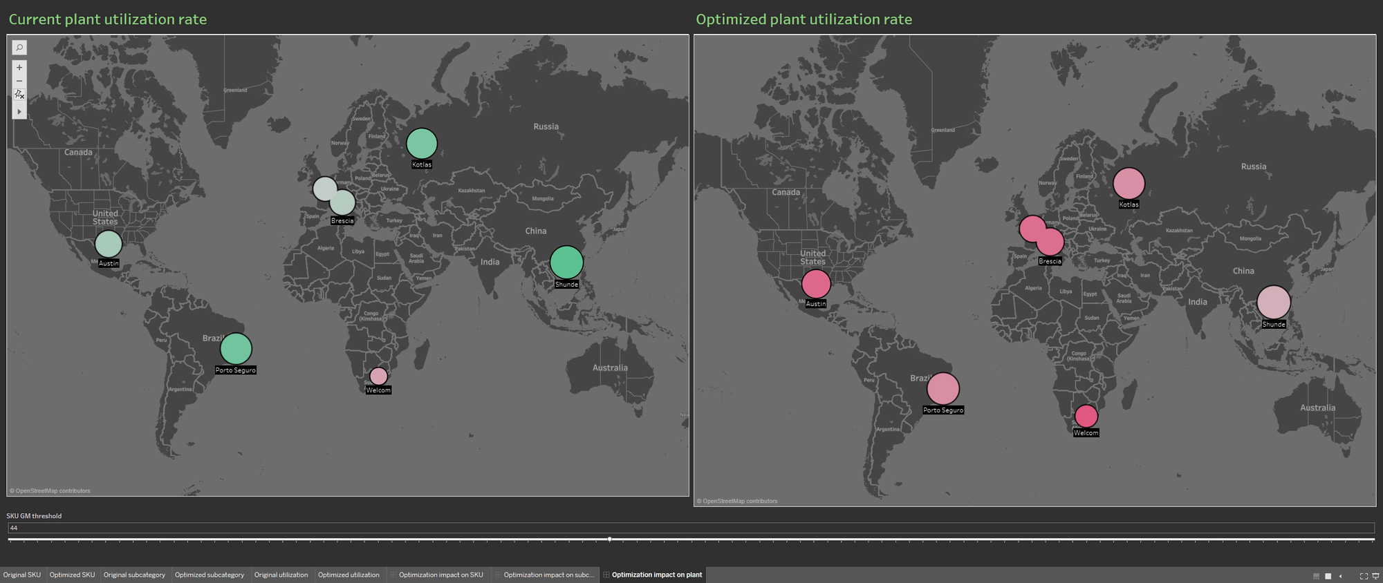
The availability of multiple data sources enriches the portfolio database by populating the visualisation with information on the current plant utilisation rate and on the rate deriving from the optimised portfolio. Again, the two information visualisations are shown side by side to better demonstrate the impact of the optimisation on the production plants.
More benefits of using TabPy within teams
In addition to the significant business value of enabling teams to interact in real time with powerful data-science techniques, this novel approach has significant back-end benefits as well. Many other data visualisation techniques require costly data scientist participation throughout the process. In this approach, however, data scientist resources are required only to prepare the draft Tableau dashboard and create the back-end Python calculation routines. Tableau’s ease of use makes it possible for a much wider range of resources to design the front end, test it with the end users and maintain it.
Front-end design is a typically a lengthy and iterative process involving multiple discussions with final users. By enabling managers to vary team composition during project execution, the novel TabPy approach can significantly improve cost efficiency. This approach also ensures high reusability of the underlying back end, enabling a wide range of users to build their own custom dashboards in Tableau to suit specific contexts, audiences and situations. This reuse of calculation logics and underlying fundamental bricks is yet another way to improve the overall cost of data visualisation.
In case you are interested in deep-diving the example, both the Tableau dashboard and Python back end are available here. If you would like additional information on this approach, please see the official TabPy Github repo or visit this Tableau Community thread.
Related stories
VizQL Data Service from Tableau: Use Your Data, Your Way
 8 August, 2024

When and How to Use Multi-fact Relationships in Tableau
 1 August, 2024

Top data books of 2021
 12 December, 2021