Tutorial
Bring Your Own Machine Learning Model(s) with Tableau Analytics Extensions API

Background
This tutorial focuses on integrating data science workflow with Tableau using Tableau Analytics Extensions API. The tutorial shows how data scientists and developers can take advantage of Analytics Extensions API to bring sophisticated analyses and machine-learning models into Tableau and enable business users to interact with these models dynamically. By having dynamic interactions with advanced models, business users can easily apply these models to their data and find the answers to their business questions quickly.
1.1 What is the Tableau Analytics Extensions API?
Today data scientists use a rapidly-evolving and diverse set of tools and platforms to build advanced analytic models, and consequently want to have flexibility in picking their own programming language and modeling tools.
After the data scientists build models, the models need to be available to business users to draw insights and make better decisions by applying these models into their business problem. As a result, corporations need to have a single platform as an enterprise standard to make this cutting-edge analysis available to everyone in the organization. This platform should enable business users not only to interact dynamically with these models, but also to build on-demand reports and find the answers to their business questions.
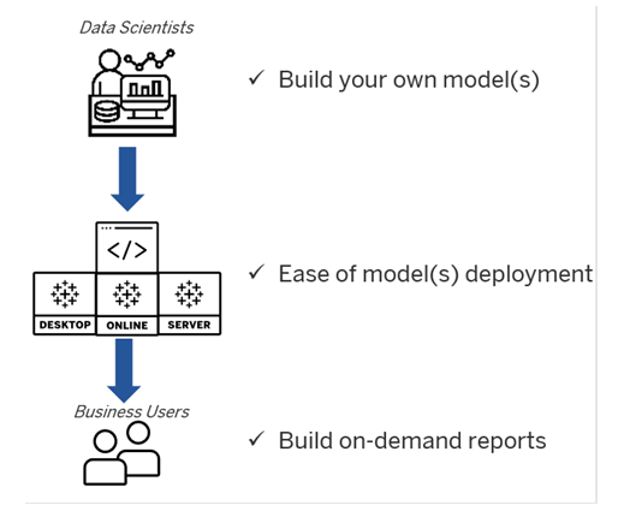
Figure 1 - Tableau Analytics Extensions API fills the gap between data scientist and business users
Tableau Analytics Extensions API was developed to meet this purpose: on one hand supporting any analytics that data scientists build with their choice of programming language, modeling tools or platform; one the other hand making these analytics available and accessible to business users.
1.2 How does Tableau Analytics Extensions API work?
The Analytics Extensions API can be employed to extend Tableau calculations to dynamically include popular programming languages and external tools and platforms. Although Tableau Analytics Extensions API was originally designed for R/Python integration, today this API has been expanded to make it more generalized for any external analytics engine. The Analytics Extensions API makes it possible to extend Tableau calculations by communicating with almost any analytics engine. These external analytics engines can receive data from Tableau and return results back in real time. The analytic engines include almost any scripting language, such as Python, R, Java, C++, as well as most of the data science platforms, such as Amazon Sagemaker, Rapidminer, and Einstein Discovery.
The focus of this tutorial is to integrate Tableau with machine-learning models built with Python. Tableau integration with Python requires TabPy, which is an open-source Python library developed and maintained by the Tableau engineering team.
TabPy can be installed like to any Python open-source library on any local computer or server such as Heroku, AWS, etc.
After installing TabPy, it needs to be run on a local computer or server. When TabPy is running, it is acting as a listener for Tableau to determine if Tableau sends any code to execute, and if it does, TabPy will run the code and send back the result to Tableau.
In addition to installing and running TabPy, users also need to configure Tableau (Desktop/Server/Online) so that Tableau knows where TabPy is running.
After setting up the Tableau configuration, users can communicate with external services from Tableau and run the Python scripts through table calculations using SCRIPT functions for expressions. There are four types of script calculations: SCRIPT_REAL SCRIPT_INTEGER, SCRIPT _STRING, and SCRIPT _BOOLEAN, which basically tell Tableau what data type to expect as a result from the analytics extension. The script functions accept aggregated dimensions and measures, and parameters. A script function passes an expression to the analytics extension and the result is returned as a table calculation. Understanding how Tableau table calculations work is vital for this integration.
2. Use Case
In this session we are going to solve a real-world business problem to find the optimum real-estate investment strategy. Solving this problem requires the dynamic interaction of multiple machine learning models. The models are built outside of Tableau with Python, and then Tableau Analytics Extensions API is used as a deployment platform to mingle the models together and make them accessible through Tableau platforms. Hence, the business users will be able to interact with these models in real time.
2.1 Business Problem
There are 223 restaurants available for sale in 12 counties of California State. The characteristics of each restaurant, such as capacity, area, food diversity, age, and price range, are available, as well as the real-estate costs.
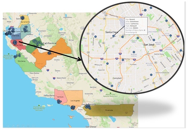
Figure 2 - Viz to show the location of available restaurants for sale at each county
In addition to the list of for-sale restaurants, information about similar restaurants is available, including their characteristics and the estimation of annual profit. The business question is this: given a budget limit, which county and restaurants are the best options for purchase/investment?
Obviously, having the real-estate cost alone is not enough to make the right decision about investment strategy, since the business goal is to maximize the long-term profitability of investment while not exceeding the investment budget.
Hence, the additional data sets can be used to inform decision-makers about the potential profitability of the restaurants available for sale. Having both real-estate and profitability data would be enough to make the right decisions.
2.2 Analytical Solutions
The analytical solution for the business problem comprises three steps, as outlined below:
2.2.1 Step 1- Building a predictive model
The first step is to build a predictive model to predict the profitability of the restaurants. The model is trained based on data from similar restaurants to learn the association and correlation between different characteristics and annual profitability. In this tutorial we are using Python with scikit-learn package to build a simple predictive model, as model building is not the main focus of this tutorial. Without going into the technical detail of model building, the following is a brief review of the steps to be taken.
Step 1-1 Reading Data
This is simply reading the data, specifying the type of variables, as well as which variable is the target to predict.
#Reading Data
url='https://raw.githubusercontent.com/AmirMK/BYOM_Tableau/main/Restaurant_profitability_data.csv'
df = pd.read_csv(url)
Target = 'Profit'
categorical_features = ['Area', 'Age', 'Type']
numerical_feature = ['Capacity_Score', 'Food_Diversity_Score', 'Price_Range']
target = 'Profit'
label=df[target]
data= df[categorical_features+numerical_feature]
Step 1-2 Data Pre-Processing
This step is to make original data ready for model building. Data pre-processing usually includes data imputation, variable scaling, converting categorical variable to numerical, etc. In general, it is a series of tasks to make original data consumable and understandable for machine-learning models.
The most important part of the data pre-processing code is to define an object containing a series of pre-processing tasks. Having all of the pre-processing tasks in one object is important, since to get the prediction for new data, the same object needs to be applied to make original data.
#Data Pre-Processing
numeric_transformer = Pipeline(steps=[('imputer', SimpleImputer(strategy='median'))
,('scaler', StandardScaler())])
categorical_transformer = OneHotEncoder(categories='auto')
encoder = ColumnTransformer(
transformers=[
('numerical', numeric_transformer, numerical_feature),
('categorical', categorical_transformer, categorical_features)])
encoder.fit(data)
Step 1-3 Model-Building and Selection
The model building process finds the model that fits best for the training data set in terms of prediction accuracy. One of the most popular approaches to achieve this goal is to iterate over multiple related machine learning models to see which one is the best fit. In this example, three regression model classes – RandomForest, K-Nearest-Neighbors (KNN) and Lasso Regression – are fitted, and the one with highest r-square is picked as the best fit.
def regressor_selection(X,y, metric = 'r2'):
pipe = Pipeline([('regressor' , RandomForestRegressor())])
param_grid = ''
param = [
{'regressor' : [RandomForestRegressor()],
'regressor__n_estimators' : [100,200,500],
'regressor__max_depth' : list( range(5,25,5) ),
'regressor__min_samples_split' : list( range(4,12,2) )
},
{'regressor' : [KNeighborsRegressor()],
'regressor__n_neighbors' : [5,10,20,30],
'regressor__p' : [1,2]
},
{
'regressor' : [Lasso(max_iter=500)],
'regressor__alpha' : [0.001,0.01,0.1,1,10,100,1000]
}
]
param_grid = param
clf = GridSearchCV(pipe, param_grid = param_grid,
cv = 5, n_jobs=-1,scoring = metric)
best_clf = clf.fit(X, y)
return(best_clf.best_params_['regressor'])
#Model Building and Selection
clf = regressor_selection(encoder.transform(data),label, metric = 'r2')
model = clf.fit(encoder.transform(data),label)
Step 1-4 Model Deployment
The model deployment step makes the machine-learning model available to make practical business decisions. Tableau Analytics Extensions API is a model agnostic platform, enabling business users to interact with any machine-learning model and make real-time decisions.
To deploy the model with Tableau Analytics Extensions API, both pre-processing objects and predictive models need to be wrapped in a single function.
def Profitability_Prediction(_arg1, _arg2, _arg3, _arg4, _arg5, _arg6):
input_data = np.column_stack([_arg1, _arg2, _arg3, _arg4, _arg5, _arg6])
X = pd.DataFrame(input_data,columns=['Area','Age','Type','Capacity_Score',
'Food_Diversity_Score','Price_Range'])
result = model.predict(encoder.transform(X))
return result.tolist()
The wrapper function simply gets the input data, applies pre-processing to make data consumable for the model, runs the model and returns the prediction. From the data-structure perspective, Tableau expects either a single value or list of values. If a list of values is used, the number of elements must match the number of rows in the calculated field that the response is assigned to.
Tableau Analytics Extensions API provides a very easy way to deploy any machine learning model. The Client method defines the TabPy connection (hostname and port number) and the deploy method is applied to persist the model on TabPy server.
from tabpy.tabpy_tools.client import Client
client = Client('http://localhost:9004/')
client.deploy('Restaurant_Profitability',
Profitability_Prediction,
'Returns prediction of profitability for restaurant(s).'
, override = True)
Step 1-5 Inference
After model deployment, the model is accessible from Tableau. Tableau users can call and query this model in real time to build on-demand reports and visualizations. Deployed models through Tableau Extensions API are available to use as table calculations in Tableau using the SCRIPT functions. In this example, SCRIPT_REAL is used because the output of deployed model returns a list of real numbers which is the prediction of annual profitability based on the restaurant's characteristic:
SCRIPT_REAL("return tabpy.query('Restaurant_Profitability',_arg1,_arg2,_arg3,_arg4,_arg5,_arg6)['response']",ATTR([Area]),ATTR([Age]),ATTR([Type]),AVG([Capacity Score]),AVG([Number of Menu Items]),AVG([Price Range]))
The following shows an interactive visualization. By selecting any county from the left-hand side, we can see the location of all restaurants in that county on the right-hand side, with their predicted profitability as label and size:
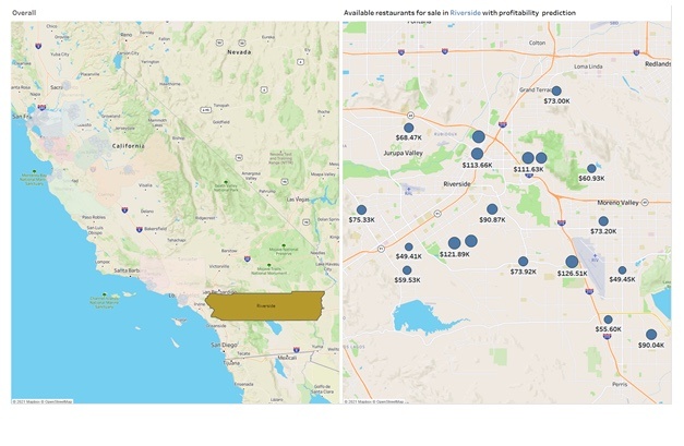
Figure 9 - Visualize the profitability prediction per restaurant
Although this viz shows the predicted profitability of restaurants individually, it would be more insightful to get the total predicted profitability at the county level. This would be a bit challenging, since any calculation field with a SCRIPT function is considered as a table calculation and is not aggregatable. One simple workaround is to use WINDOW_X functions. Although the most granular level of data still needs to be presented in the viz (i.e., restaurant), a visualization can be built in a way to show the result at county level.
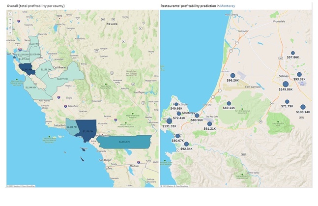
Figure 10 - Visualize the profitability prediction per restaurant and total profitability per county
In the new viz, the right-hand side view shows which county has the most predicted profitability, and by selecting each county then in the left-hand side, we can see the restaurant level prediction:
2.2.2 Step 2 Optimize the investment strategy
So far, the real-estate cost of restaurants as well as the predicted profitability are available to help business users to make a decision about which county and which restaurants are the best to invest in.
There are many heuristic methods such as Greedy method which can be used to find an answer to this question. However, this is not necessarily the global optimum decision.
The detailed business question is this: which restaurants within a county should be selected to invest to maximize profit while making sure the total real-estate cost is less than our budget?
From the analytical perspective, this problem falls into the class of optimization called Knapsack Problem. Fortunately, there are many Python packages available to solve this problem. In this example, Knapsack-pip Python library is used to find the optimum investment strategy. This is a very easy-to-use package using a branch and bound algorithm to solve the knapsack problem.
The Python code can be directly used in Tableau as a calculation field:
SCRIPT_REAL("from knapsack01.BBKnapsack import BBKnapsackProfit = _arg1Cost = _arg2Budget = _arg3[0]optimum_profit,solution = BBKnapsack(Budget, Profit, Cost).maximize()return solution",[Profit Prediction],SUM([Cost]),[Total Budget])
The main power of this integration is the fact that the input values for this analytics extension are coming directly from visualization, so the user can control and change the inputs dynamically by applying different filters on the datasets. The Python code requires three arguments as input:
-
_arg1: Refers to the first element, which is the profitability of each restaurant on the viz. This field is a table calculation and is considered as an aggregated field.
-
_arg2: Refers to the second element, which is the real-estate cost of restaurants. This field exists in the original dataset and needs to be aggregated to pass to SCRIPT functions. It must be noted the level of aggregation depends on the viz marks. In this example, each mark on the viz is a restaurant.
-
_arg3: Refers to the third element which is the total available budget for investment, which is a dynamic parameter.
The Python code output is the list of two elements:
-
Solution: Indicate True (1) or False (0) if a restaurant is selected for investment or not.
-
Optimum Profit: a single number that indicates the optimum profitability, corresponding to the solution.
To visualize the optimum investment strategy, the first element of optimization solution needs to be returned to the Tableau. The second element can also be returned in a separate calculation field to get the optimum profit.
In the new viz, the left-hand side shows the optimum profitability, corresponding to each county. By selecting each county, the right-hand side will show the best investment strategy, that is, which restaurants to buy or invest in.
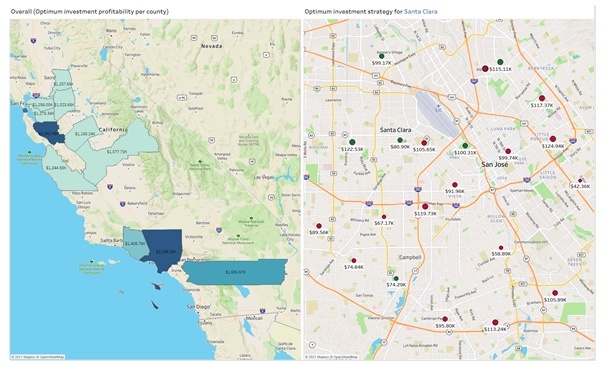
Figure 12 - Visualize the optimum investment strategy per county
3. Why real-time solution?
There are many factors which might impact the decision-making process, and most of the time, these factors are dynamic. As a result, the business users need to be able to interact with the machine-learning model in real time to get the best answer considering the current business circumstances.
In the above example, one of the primary factors which impacts the result of investment strategy is the budget limit. Although the budget limit was assumed to be fixed, in the real world, business users want to try different scenarios to see how increase or decrease the investment budget would impact the investment profitability and strategy. In such a situation, having an effective interaction with the model is a vital part to finding the right answer to the right question(s). From the analytical perspective this analysis is known as sensitivity analysis or what-is analysis, which helps users to understand the impact of parameters on the output.
For example, a new report can be built to examine the impact of changing the budget limit and can be used for what-if analysis. In this example, it seems increasing the investment budget by 25% from $8M to $10M will lead to 30% increase in profitability:
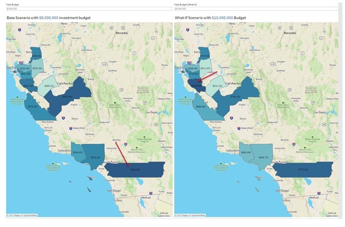
Figure 13 - What-if/sensitivity analysis over investment budget limit
Another example of real-time interaction with a model is the situation in which some of the restaurants will be taken off the market. In Tableau, a related filter can easily be applied to the viz to exclude the off-the-market restaurants and you can easily re-run the model to get real-time results.
4. Wrap-Up
This tutorial demonstrated how Tableau Analytics Extensions API can be employed as a deployment platform to fill the gap between data scientists ,developers and business users. Once an advanced analytics model is deployed, business users can easily apply these models to their data and find the answers to their business question quickly.
5. Troubleshoot
Business users might observe some performance issues while building the visualization with a Tableau calculation field that includes Python code or other external service integration. As mentioned earlier, a calculated field with a SCRIPT function is considered a table calculation, so defining the right dimensions is vital for good performance.
5.1 Prediction
By dragging the ‘Profit Prediction’ field into the visualization, Tableau, by default, sets the dimension at the mark level. In other words, for each mark Tableau calls the deployed function. For example, if there are 10 restaurants in the viz, there will be 10 calls to the deployed function, which can cause some performance issues. To avoid such a problems, user can specify the dimension at the Zip Code level (which is identical for each restaurant). As a result, Tableau will not partition the data and will send all data at once, so there is just one call to the deployed model, which is more efficient.
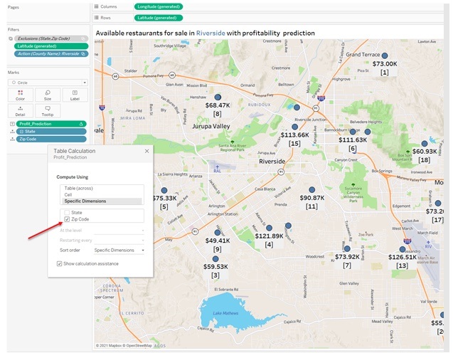
Figure 14 - Set the right prediction dimension to avoid performance issue
5.2 Optimization
Similar to the issue with the prediction model, by dragging the ‘Optimized Profit’ field into the visualization, Tableau, by default, sets the dimension at the mark level. However, in this case the performance is not the only issue, but also the results of optimization. In this case, Tableau basically runs the optimization for each restaurant separately, while the goal is to run the optimization for all of restaurants within each county together. Hence the table calculation dimension needs to be adjusted to Zip Code while make sure County is part of the viz detail.
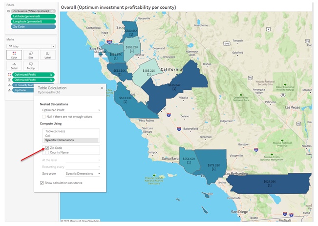
Figure 15 - Set the right optimization dimension to avoid wrong result
By this adjustment Tableau partitions the data based on county, so the optimization will run for all restaurant together per county separately.
Question: What would happen if ‘County Name’ be selected dimension as well? Why the result would be wrong?
6. Further Reading
All material related to this content including data set, Python code and Tableau workbook can be found in this link. You can replicate the same examples, or make adjustments and changes to customize it with your own dataset or similar use cases. The example in this tutorial primarily focused on a supervised machine learning models and optimization. If you are interested in learning how Tableau Analytics Extensions API can bring in other types of machine learning models, such as unsupervised learning, see this article about Applying Clustering Analysis.
Last updated: 03 October, 2021