Exploring Spatial Relationships in Tableau


Sarah Battersby was a member of Tableau Research from 2015-2023, with a primary focus on cartography, and emphasis on cognition. Sarah holds a PhD in GIScience from the University of California at Santa Barbara, and is a member of the International Cartographic Association Commission on Map Projections, and is a past president of the Cartography and Geographic Information Society (CaGIS). Connect with Sarah at @mapsOverlord and explore her work on Tableau Public.
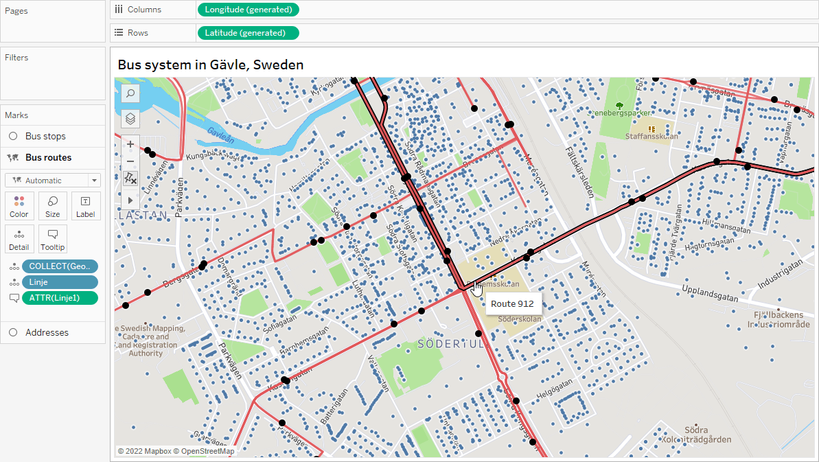
Maps are a great tool to visually analyze spatial patterns. In Tableau, it’s simple to add multiple layers of data on top of a custom base map to easily see patterns. In the example below, identifying all of the bus routes (red), bus stops (black points), and address locations (blue points) is effortless.
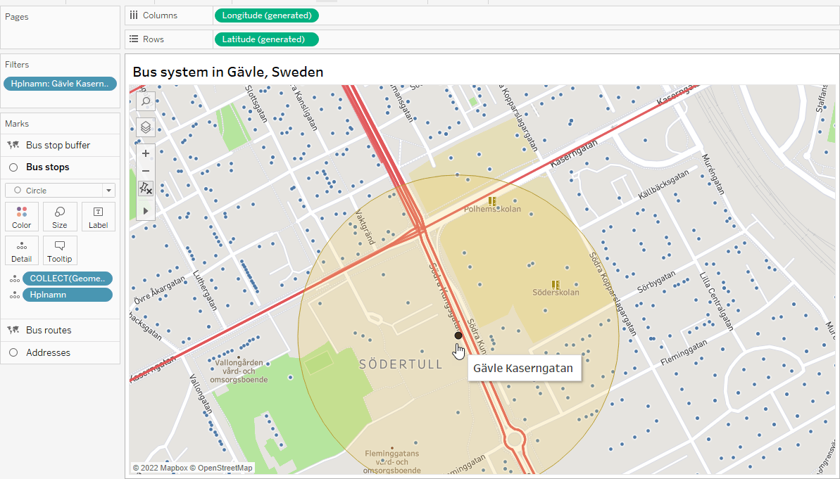
But sometimes you need to go beyond seeing the relationship between your data sets and quantify exactly how they relate to each other. For instance, what if we wanted to explore the accessibility of different bus lines and needed to know exactly how many addresses were within walking distance of each bus stop? We can quickly visualize it by adding a buffer around the bus stops so we can see which points are inside the buffer.
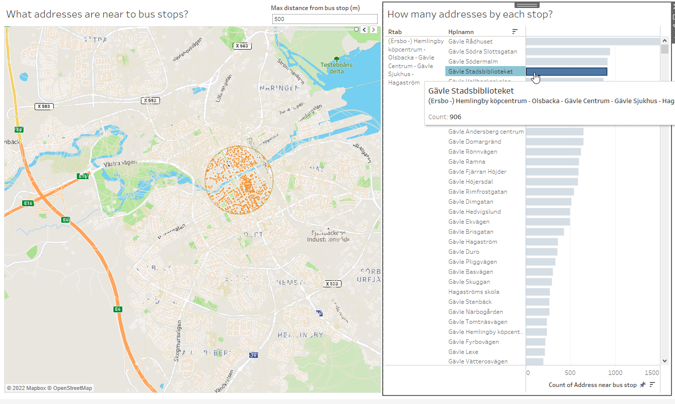
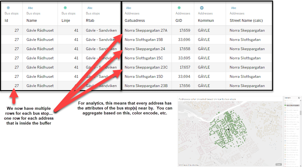
We can also quantify the results using Tableau’s spatial intersection joins and calculations to allow interactive analytics. In the example below, we can see addresses within a user-defined distance of each bus stop, and we can quickly highlight the data related to any individual location of interest.
Setting this up in Tableau is easy. We just need to use a spatial join to define the relationship between our data sets and then set up a few quick calculations to draw our buffers and color encode the nearby points.
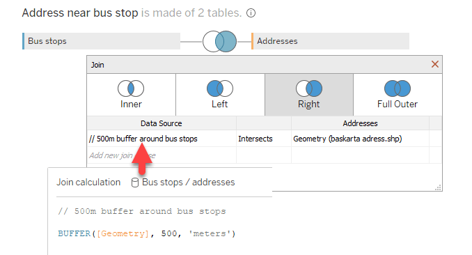
The spatial join is based on a 500 m buffer around each of the bus stops and the point geometry for the addresses. Tableau checks to see which address points fall inside that 500 m buffer polygon and sets up the spatial relationship we need to answer our questions.
Now the data sets have a spatial connection between them.
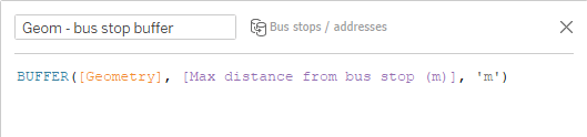
Once we have that join set up, we can use a quick calculated field to make a graphical buffer to visualize on the map. Notice that the calculation below doesn’t use the same 500 m distance; it uses a parameter instead. As long as that distance parameter is smaller than the one in the spatial join above, we can dynamically adjust how far we search in our analyses.
Now we just need a calculation that returns a boolean (True/False) on whether or not the address is within the threshold set by our maximum distance parameter.
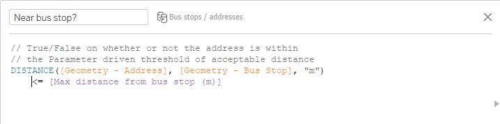
Now we have a user-controlled, dynamic map to quantitatively explore what is “near by” to our bus stop locations of interest.
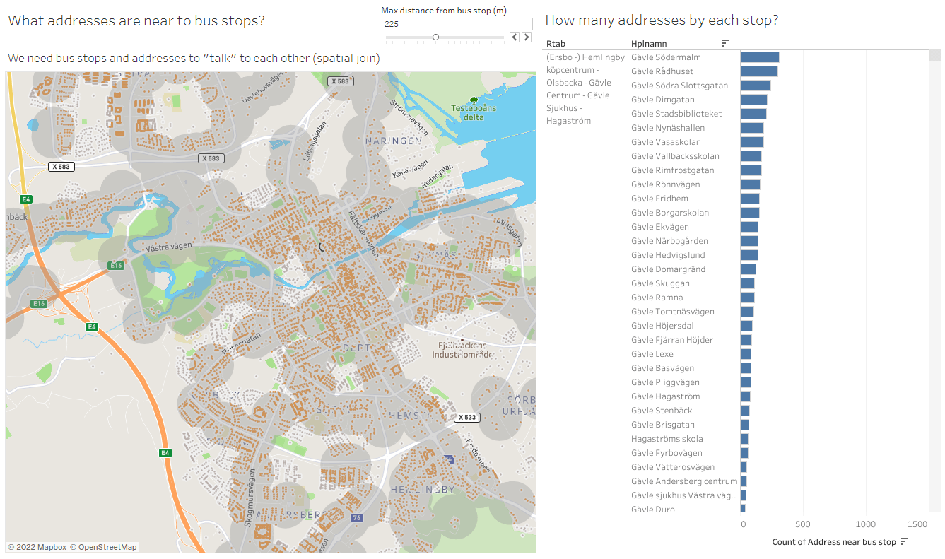
The spatial joins between data sets can be used to answer all sorts of interesting questions, including things like finding all bus stops and routes served by those stops within the distance of a single address of interest.
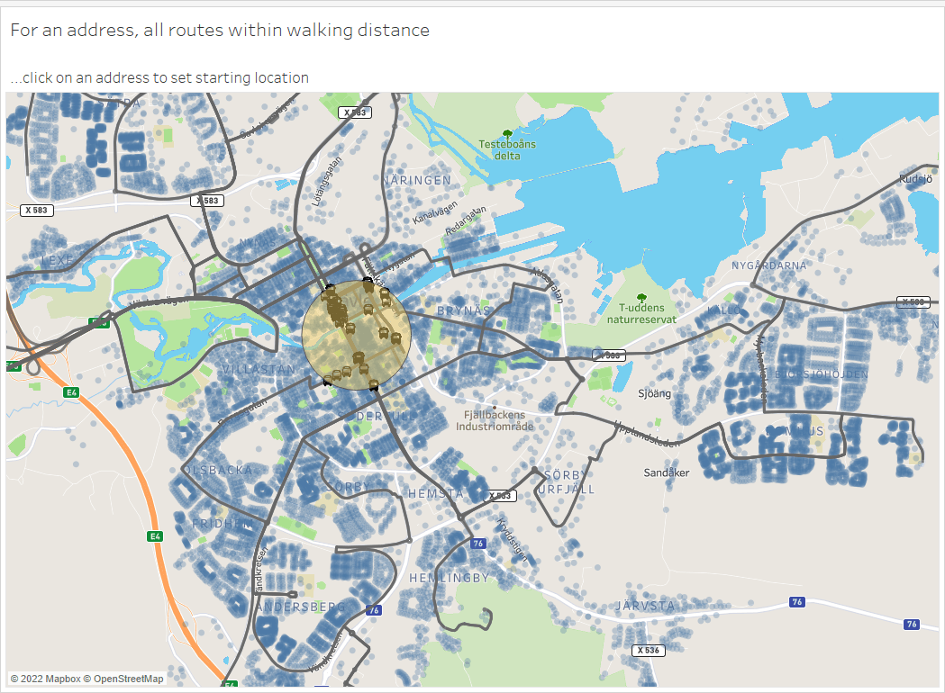
Spatial interactions in Tableau work with most combinations of point, line, and polygon geometries, so the possibilities for getting your spatial data files “talking” to each other are virtually limitless.
Storie correlate

A Guide to Mapping and Geographical Analysis in Tableau
 15 Novembre, 2024

Spatial Parameters and Calculations: Make More Dynamic, Interactive Maps
 18 Ottobre, 2024
How Maps Help Us Understand the World
 8 Luglio, 2022