Streaming Analytics with Tableau and Databricks


Many companies struggle to bring streaming data into their customer experiences and to deliver real-time decision-making to all employees. A recent IDC survey found that less than 25% of organizations had adopted data streaming enterprise-wide. Most could only implement data streaming for one-off use cases with brute force from highly specialized resources and technology. Streaming data projects were typically expensive and hard—with new APIs and languages to learn and separate systems and operational tooling.
To reduce complexity, organizations are turning to lakehouse architectures, which bring streaming and batch data sets into a common platform that can serve the needs of live interactive analytics, machine learning, and real-time applications. Databricks has emerged at the forefront of delivering this lakehouse paradigm. The Databricks Lakehouse Platform combines the qualities of data warehouses and data lakes to provide:
- The ability to build streaming pipelines and applications faster
- Simplified operations from automated tooling
- Unified governance for real-time and historical data
Databricks and Tableau have delivered a number of innovations that make it possible to provide responsive, scalable performance when analyzing streaming data:
- Tableau enables live connectivity to lakehouse data sources with no loss of analytical functionality. You can seamlessly toggle between in-memory extracts and live connectivity at the data source level without updating any downstream workbooks. This facilitates rapid experimentation and helps to accelerate the adoption of real-time data sources. By contrast, most BI tools offer reduced functionality when using live connections.
- Databricks SQL is a serverless data warehouse that enables you to provision specialized compute resources, optimized for live analytics. This helps overcome limitations with many data lake query engines which provided good throughput but struggled to scale to high concurrency. Databricks SQL offers more concurrency through automatic load balancing, caching, query optimization, and the next-generation Photon vectorized query engine.
- Tableau live connections to Databricks SQL warehouse clusters also feel much more responsive when exploring data due to query scheduling improvements. We no longer see contention with the mix of metadata queries, fast queries and long-running queries that are typical for live exploration.
How should I structure agile data sprints?
Today many data projects are still structured in a linear fashion: the data engineering team spends time acquiring and harmonizing data, and then business domain experts are involved relatively late to explore, develop insights, and integrate into application workflow. However, agile data sprints should be run in an iterative way that involves business domain experts early:
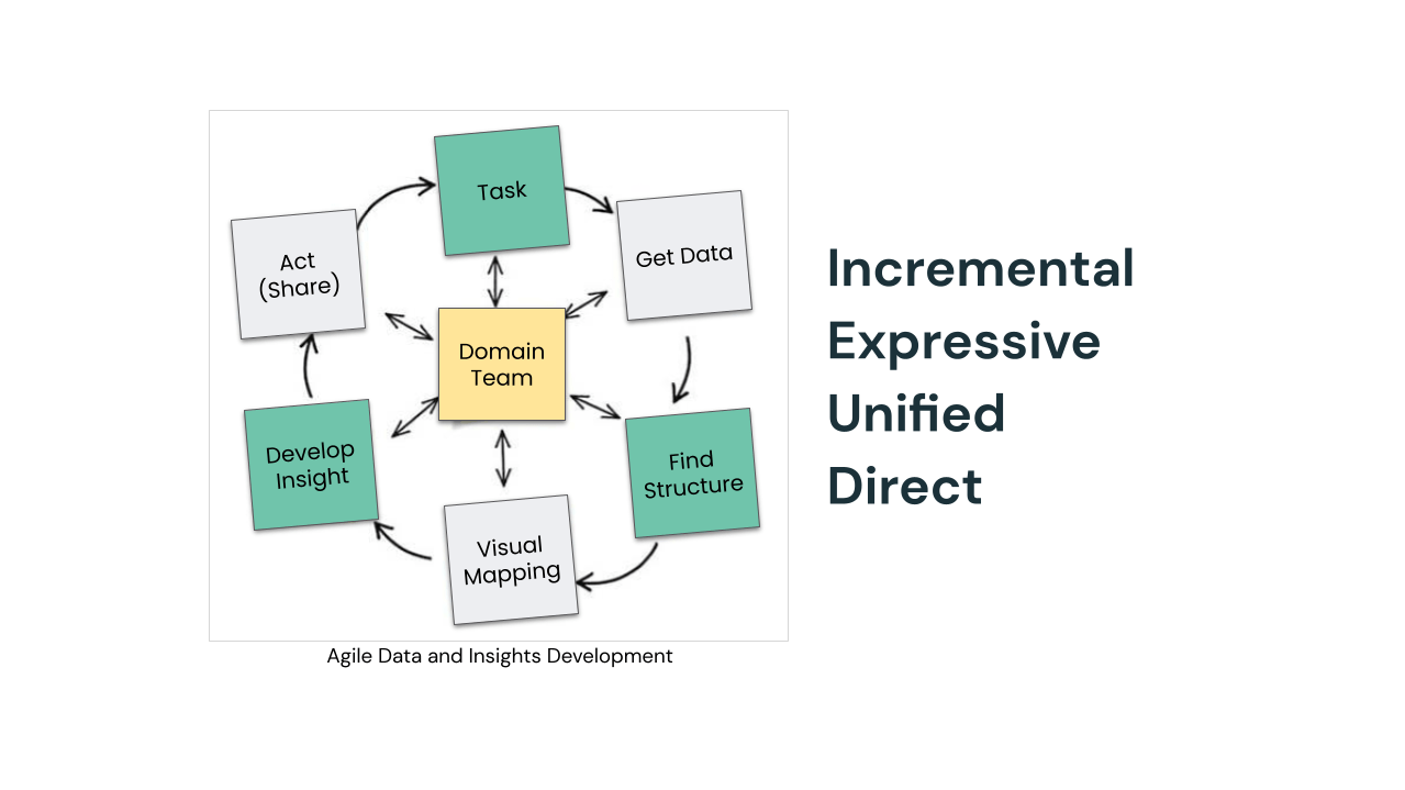
We often find that once business users start to develop insights, we need to go back and acquire more data, or fix quality issues, or adjust the structure to fit the business domain. One of the benefits of a data lakehouse is the ability to reduce the number of hops and flatten out the data pipeline; however, we don’t tap into that benefit unless we adopt new ways of working. When we structure these projects as short agile sprints, the whole domain team is encouraged to continue to ask deeper and deeper questions, and we lower the cost of curiosity.
In this cookbook we will break down a streaming data project into three steps:
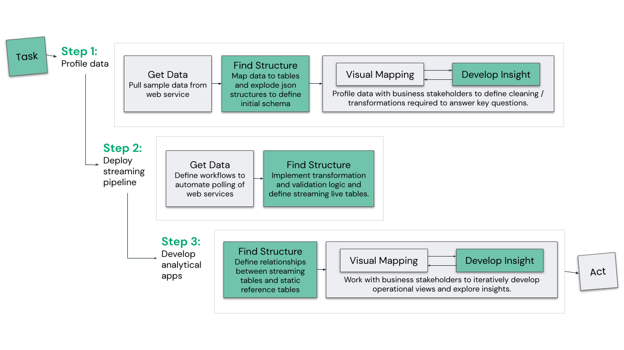
Step 1: Profile Data
The data engineering team quickly exposes a sample subset of the streaming data source to business domain experts for data profiling. The team uses Tableau to identify missing data or data quality issues and to run experiments to determine if the data needs to be restructured to be able to easily answer questions.
Step 2: Deploy streaming pipeline
Having agreed on data-cleaning business logic and the right schema for analytical data sets, the data engineers use Delta Live Tables to declaratively build a streaming data pipeline to continuously ingest, clean and transform the data.
Step 3: Deploy analytical apps
Business domain experts can now connect live to the analytical data sets using Tableau and define views, dashboards, data alerts and workflows to operationalize the data.
Implementation Cookbook
In this example, we will poll the Divvy Bikes Data Service at regular intervals and write the results to cloud object storage to generate the input stream for our analysis. This is a useful design pattern for fetching near real-time updates from REST services, but if you need to ingest data directly from an event bus or a messaging system then it is worth reviewing this blog which describes the syntax for ingesting data directly from Kafka and similar services.
End-to-End Data Pipeline
This cookbook will show how to configure the following services to enable real-time analytics:
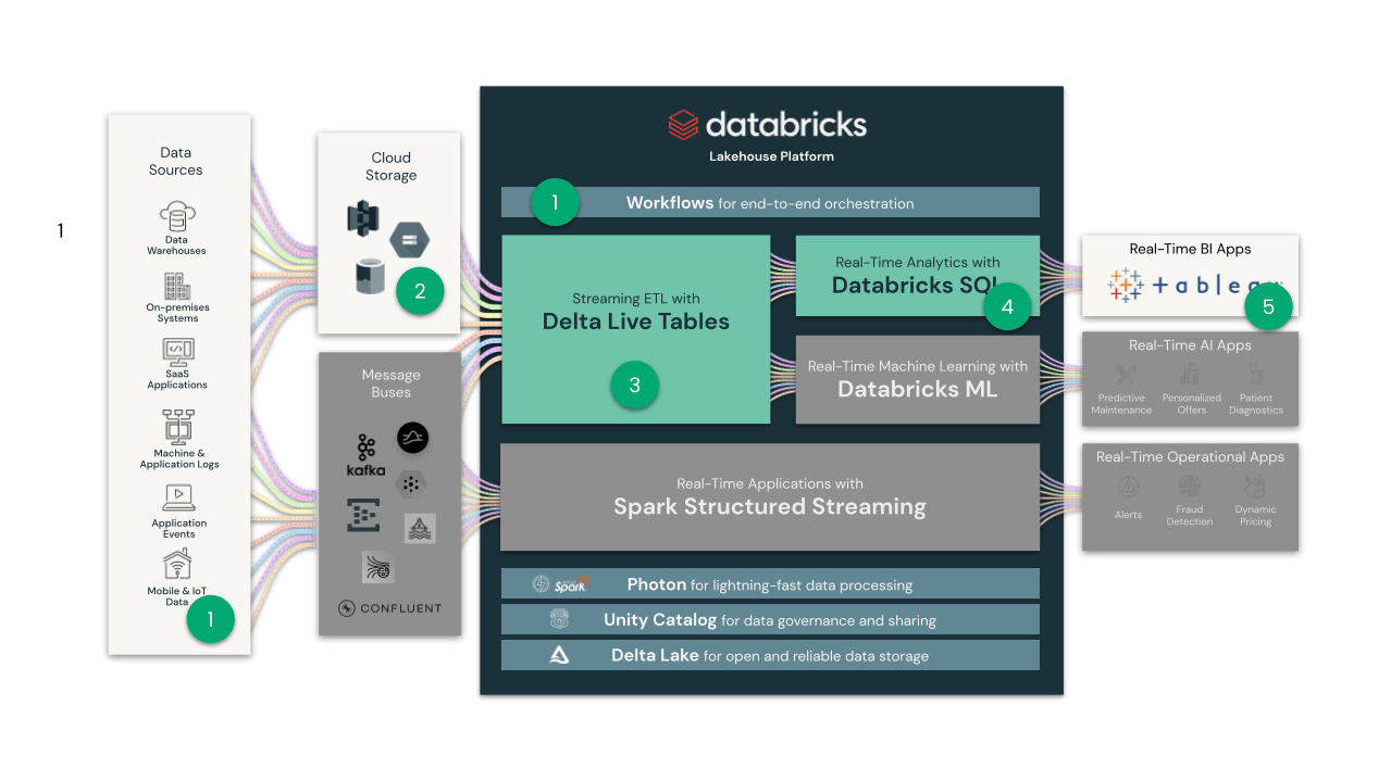
- We will define a Databricks Workflow to poll an IoT Service at regular intervals to check device status.
- This raw status data will be output to Cloud Storage.
- We will declaratively define Delta Live Tables to continuously ingest and transform/clean the raw status data.
- We will expose the live streaming tables to Tableau via a SQL Warehouse endpoint.
- We will explore the data in Tableau through a live connection and derive some initial insights.
Source Notebooks
View the full source notebooks for each step outlined in this session.
Step 1: Profile Data and Define Structure
1.1 - Get Data
The data used in this example is provided in JSON format by a public data service. We create a simple notebook to poll the data service and output this to cloud storage. In a later step, we will schedule this notebook to run at regular intervals to create a continuous input stream so we ensure that each run will emit a unique filename:
import os, time
import requests, json
from datetime import datetime
# get current timestamp
now = datetime.now()
fmt_now = now.strftime("%Y%m%d_%H-%M-%S")
# get json response from api
station_status_url = "https://gbfs.divvybikes.com/gbfs/en/station_status.json"
resp = requests.get(station_status_url)
resp_json_str = resp.content.decode("utf-8")
# write response to cloud storage
api_resp_path = '/Shared/DivvyBikes/api_response/bike_status'
with open(f"/dbfs/{api_resp_path}/bike_status_{fmt_now}.json","w") as f:
f.write(resp_json_str)
1.2 - Find Structure
In order to analyze the bike status data we need to take the semi-structured API response and transform it into a well-structured schema.
First, we load the raw bike status data into a table. Note that the “path=” syntax below will load all json files from the input directory:
CREATE SCHEMA IF NOT EXISTS divvy_exploration;
CREATE TABLE divvy_exploration.bike_status
USING json
OPTIONS (path="/Shared/DivvyBikes/api_response/bike_status")
Each file in the input directory will be loaded as a single line in the import table. We examine the json structure to make an initial determination of which fields we need to bring into our target schema:
Next, we transform the nested JSON structures into tables for analysis. In this example our source structure is two levels deep so we need to first explode the stations list before we can extract fields from each station object:
CREATE TABLE divvy_exploration.bike_status_flattened AS
SELECT
stations.station_id,
stations.num_bikes_available,
stations.num_bikes_disabled,
stations.num_docks_available,
stations.num_docks_disabled,
stations.num_ebikes_available,
stations.station_status,
stations.is_renting,
stations.is_returning,
CAST(stations.last_reported AS timestamp) AS last_reported_ts
FROM
(
SELECT
EXPLODE(data.stations) AS stations
FROM divvy_exploration.bike_status
)
Our flattened data is now ready for data profiling in Tableau:
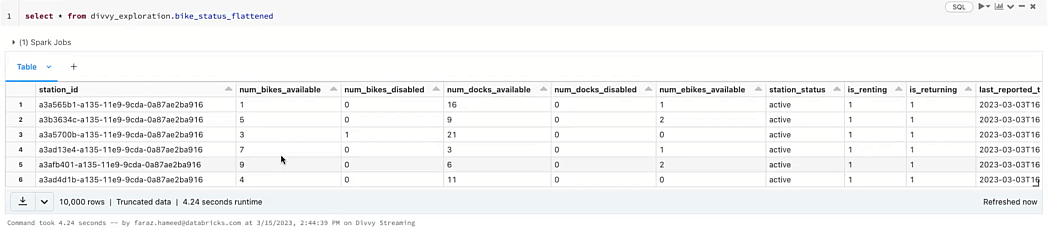
1.3 - Data Profiling
You can explore these tables with Tableau by connecting directly to the all-purpose Databricks cluster that we used to import and transform the data. However, we recommend you define a Databricks SQL Warehouse which provides specialist compute resources that are optimized for live analytics. We recommend you use a Pro or SQL Serverless Warehouse Type in order to access the full set of performance optimizations. This will provide better concurrency and responsiveness as we scale the insights to more business users. All compute clusters operate against the same datasets so this provides workload isolation without requiring additional data copies or introducing data freshness concerns.
The simplest way to manage authentication is by generating a personal access token. You can connect to Databricks directly from the Tableau Cloud or Tableau Server web authoring experience using the native connector. The following diagram shows where to obtain each of the required connection details:
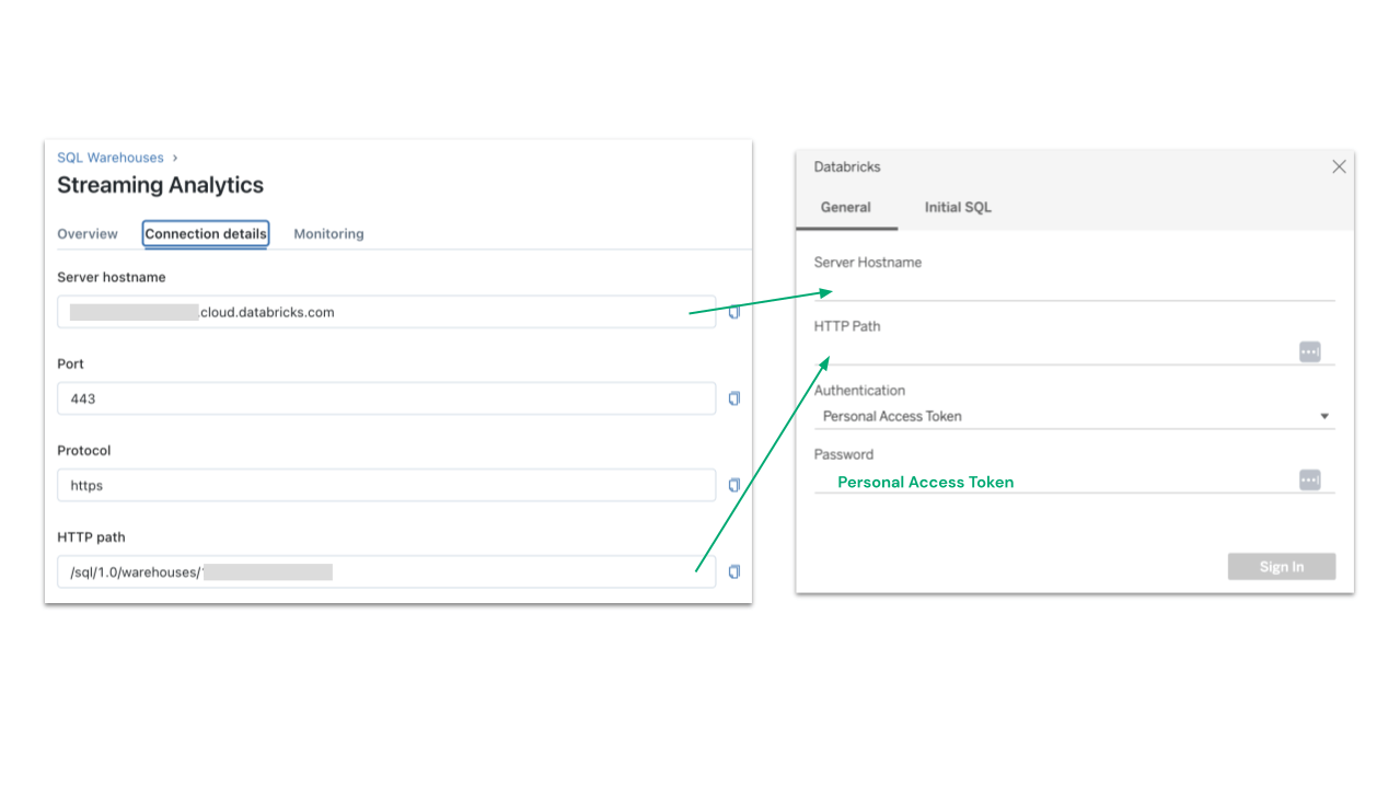
Once you have connected to the sample data you should engage with your business domain experts to explore the data in Tableau. At this stage the following baseline checks are typically performed using visual analysis:
- Data Conformity - Check for NULLs and out-of-bounds values.
- Data Completeness - Validate that the live streaming data is reporting status updates for each of the expected entities (in this example we check the number of status updates in the bike_status table against the stations listed in the station_information reference table).
- Data Currency - Check that the data from all entities are up-to-date
These checks will define the data cleaning business logic that needs to be implemented in the streaming data pipeline.
The domain team also works together to validate that the table structure can efficiently answer their questions (business domain alignment) and identify that all required fields are present in the sample dataset (while parsing the JSON entities we only retained a subset of the available fields).
Step 2: Deploy Streaming Data Pipeline
2.1 - Schedule IoT Data Polling at regular intervals
Databricks Workflows provide an orchestration service that we can use to schedule the notebook defined in Step 1.1. For this example we will poll every five minutes. This step is not required if attaching directly to a service like Kafka.
2.2 - Implement Data Validation and Cleaning Logic
Delta Live Tables provides a declarative framework to define transformations, data validation rules and target structure. You can use SQL syntax to declare a continuous pipeline as shown below:
-- Create the bronze bike status table containing the raw JSON
CREATE TEMPORARY STREAMING LIVE TABLE bike_status_bronze
COMMENT "The raw bike status data, ingested from /FileStore/DivvyBikes/api_response/station_status."
TBLPROPERTIES ("quality" = "bronze")
AS
SELECT * FROM cloud_files("/FileStore/Shared/DivvyBikes/api_response/bike_status", "json", map("cloudFiles.inferColumnTypes", "true"));
-- Create the silver station status table by exploding on station and picking the desired fields.
CREATE STREAMING LIVE TABLE bike_status_silver (
CONSTRAINT exclude_dead_stations EXPECT (last_reported_ts > '2023-03-01') ON VIOLATION DROP ROW
)
COMMENT "The cleaned bike status data with working stations only."
TBLPROPERTIES ("quality" = "silver")
AS
SELECT
stations.station_id,
stations.num_bikes_available,
stations.num_bikes_disabled,
stations.num_docks_available,
stations.num_docks_disabled,
stations.num_ebikes_available,
stations.station_status,
stations.is_renting,
stations.is_returning,
last_updated_ts,
CAST(stations.last_reported AS timestamp) AS last_reported_ts
FROM (
SELECT
EXPLODE(data.stations) AS stations,
last_updated,
CAST(last_updated AS timestamp) AS last_updated_ts
FROM STREAM(LIVE.bike_status_bronze)
);
Note that this definition builds on top of the table definitions from step 1.3 but we now also add data validation constraints.
2.3 - Deploy Streaming Live Table
When you run the above statements Databricks validates the syntax and returns the following message on success:
This Delta Live Tables query is syntactically valid, but you must create a pipeline in order to define and populate your table.
This definition is now used to build delta live tables as shown here. We recommend that you initially schedule this as “triggered” rather than “continuous”. You can then review output and identify data quality issues before converting to continuous execution.
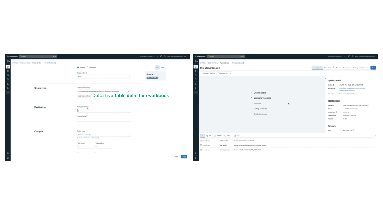
Once the pipeline is deployed review the topology, status and data quality logs to confirm all is working as expected:
Step 3: Develop Analytical Applications
3.1 - Connect to a Streaming Live Table from Tableau
We can now connect to the Delta Live Tables with the same SQL Warehouse connection that we used to profile the data. The streaming tables behave like regular tables but are continuously updated as changes arrive in the S3 source (or streaming service).
3.2 - An example analytical application
As we are using a live connection we push all query processing down to Databricks SQL and can therefore explore and rapidly prototype against very large and complex datasets. The domain team can work together using Tableau to derive insights in an incremental, expressive, unified and direct way and then scale those views to the whole organization. If data changes are required then we can quickly iterate to update the streaming data pipeline using Delta Live Tables’ declarative framework.
Next Steps
We hope you’ve found this methodology and walkthrough useful in getting your streaming analytics project up and running. Interested in learning more? Check out the Intro to Streaming Analytics webinar, where we walked through this end to end process live.
Source: IDC Streaming Data Pipeline Survey, December 2021
Articles sur des sujets connexes
Tableau and dbt Labs: Strategic Partnership and Integration
 août 25, 2025

Supercharge Analytics with the Power of AWS-Hosted TabPy
 octobre 14, 2024
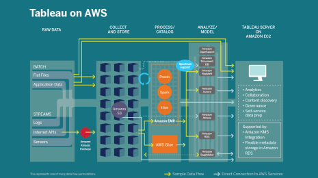
Tableau + AWS: Accelerating your digital transformation with Modern Cloud Analytics
 novembre 27, 2023
Tableau and AWS help customers digitally transform with Modern Cloud Analytics, combining technical resources and expertise with our vast partner networks.