A Handy Guide to Choosing the Right Calculation for Your Question


Tableau has multiple forms of calculation. And for those who are new to Tableau, choosing the right type of calculation to employ for a given problem can pose a challenge.
Let's first lay out the types of calculations:
Basic calculations: These calculations are written as part of the query created by Tableau and therefore are done in the underlying data source. They can be performed either at the granularity of the data source (a row-level calculation) or at the level of detail of the visualisation (an aggregate calculation).
Level of Detail Expressions: Like basic calculations, LOD Expressions are also written as part of the query created by Tableau and therefore are done in the data source.
The difference is that LOD Expressions can operate at a granularity other than that of the data source or the visualisation. They can be performed at a more granular level (via INCLUDE), a less granular level (via EXCLUDE) or an entirely independent level (via FIXED).
Table calculations: Table calculations are performed after the query returns and therefore can only operate over values that are in the query result set.
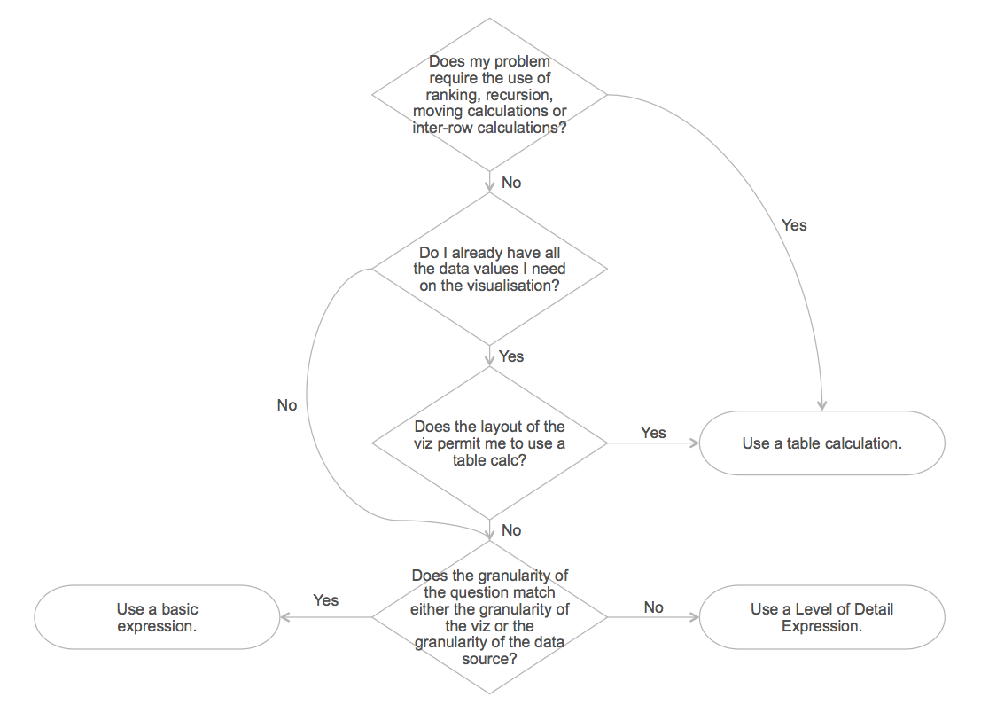
So how do you choose the right calculation? Let's compare the different calculations types.
1. Basic Calculation vs. Table Calculation
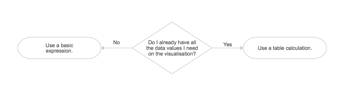
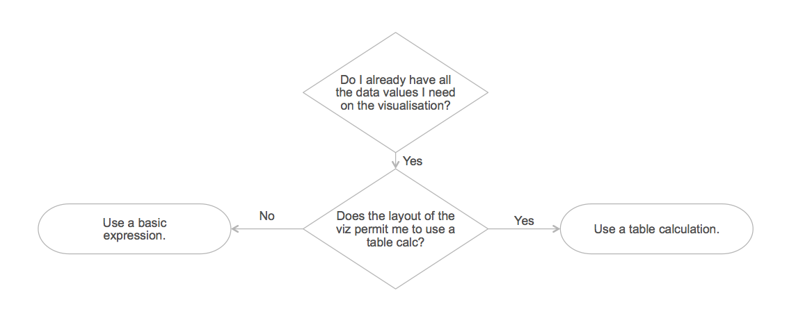
When trying to choose between basic calculations and table calculations, the important question is: Do I already have all the data values I need on the visualisation?
If the answer is yes, then you can calculate the answer without further interaction with the data source. This will often be faster as there is less data that needs to be processed (i.e. we are just computing using the aggregated values from the result set).
If you do not, then you have no choice but to go to the underlying data source to calculate the answer.
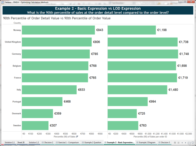
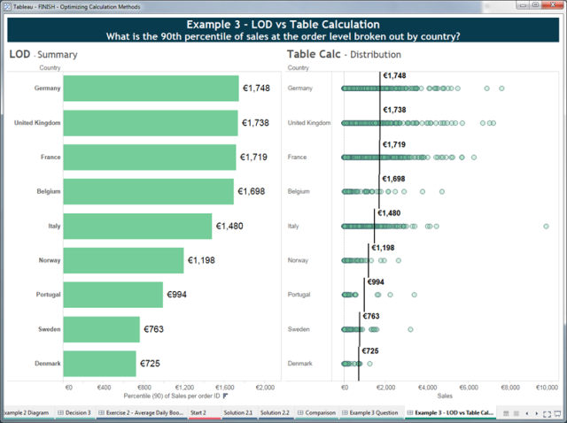
Consider the following example in which we ask: What is the 90th percentile of our order details, shown by country?
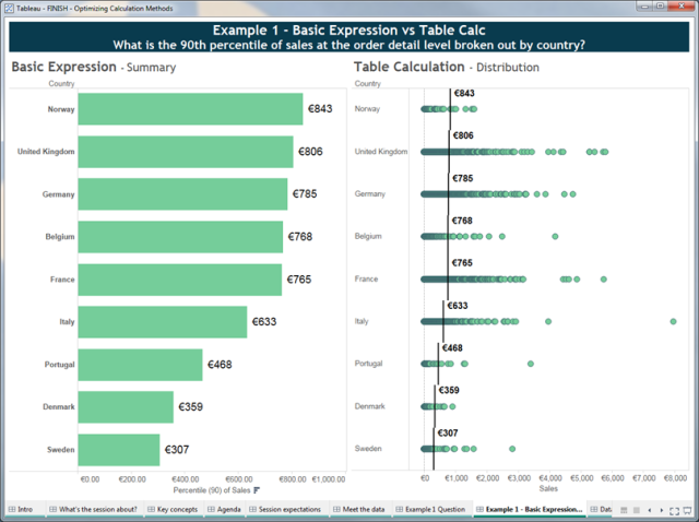
Both sides of this dashboard answer the question. If you were just interested in the 90th percentile value and didn’t need to determine further insights, then the chart on the left would be optimal. It provides a minimal result set (one number per country) via a basic aggregation PCT90([Sales]) which is calculated in the underlying data source.
However, if you wanted to gain further insights (e.g. understand the greater distribution and identify outliers) or add other aggregations (e.g. you also wanted the median values) then the chart on the right allows you to do that without further queries. The initial query to return all the order detail records (the green dots) provides all the data necessary to locally compute the 90th percentile as well as explore other insights.
One of the key takeaways from this post is that the layout of the viz matters. As we’ve already discussed above, the viz design will impact how much data you initially return from the data source. This is an important factor in determining your approach.
However, there are situations where, although you have all the data you need in your result set, it is not possible to achieve the required layout using a table calculation. So you also need to ask: Does the layout of the viz permit me to use a table calc?
Consider the following example in which we ask for the year-over-year difference in sales in two formats, one as a chart and the other as a table:
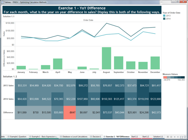
The top half of this dashboard is easily achieved using a table calculation. Simply duplicate the Sales field and apply a difference quick-table calculation run across the Order Date dimension. However, if you try to then convert that computation structure into a table, you end up with the following:
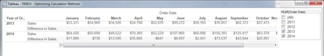
You will realise that it’s not possible to achieve the specified layout with a table calculation as you need the Year dimension with the Measure Names dimension nested inside. Tableau cannot suppress the “Difference in Sales” row for 2013. So in this example, your only option is to use basic calculations:
[2013 Sales]
IF YEAR([Order Date]) = 2013 THEN [Sales] END
[2014 Sales]
IF YEAR([Order Date]) = 2014 THEN [Sales] END
[Difference]
SUM([2014 Sales]) – SUM([2013 Sales])
This approach allows you to just have the Measure Names dimension which you can sort to meet the layout requirements.
2. Basic Calculation vs. Level of Detail Expression
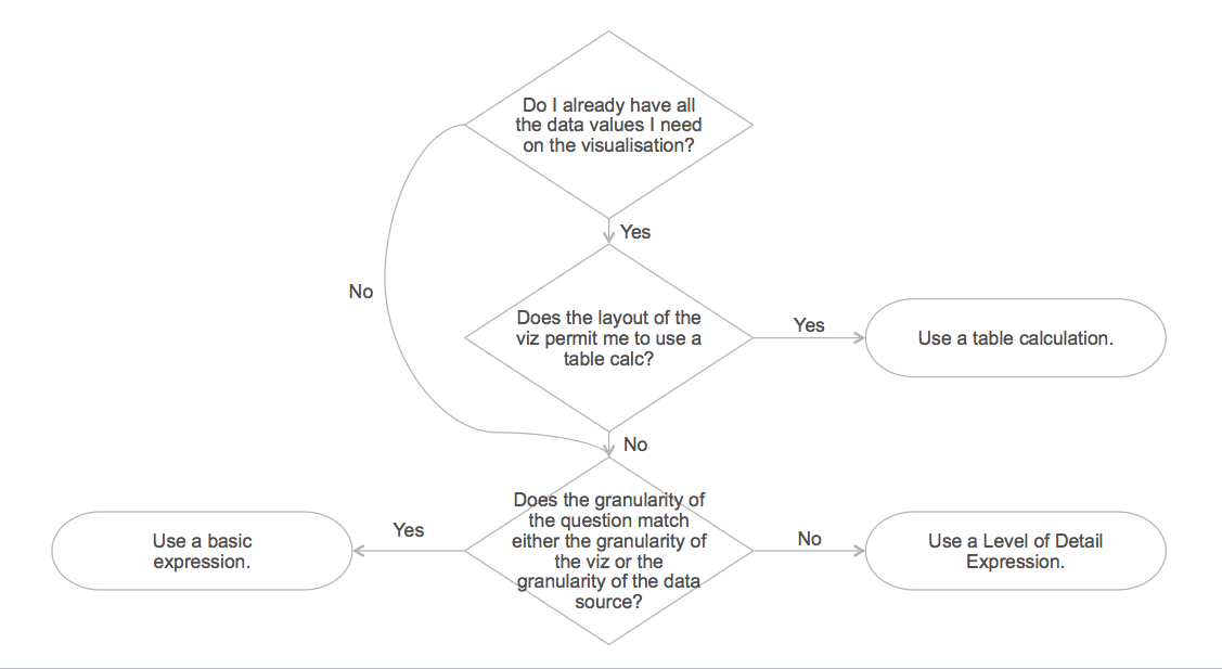
If we do not have all the data we need on the visualisation, we need our calculation to be passed through to the data source. This means we must use a basic calculation or an LOD Expression.
But how to choose? The important question to ask here is: Does the granularity of the question match either the granularity of the viz or the granularity of the data source?
Basic calculations can be performed either as row-level calculations or as aggregate calculations. So they can only answer questions at the granularity of the data source or at the level of detail of the visualisation. Level of Detail Expressions, on the other hand, can answer questions at any granularity.
Consider the following example in which we ask: What is the 90th percentile of sales at the order-detail level compared to the order-total level?
If you are familiar with the superstore data set (which ships with Tableau), you will know that it is one row of data per line item of each order. So if we consider the question above, we determine:
- Granularity of data source: Order Detail
- Granularity of viz: Country
- Granularity of left chart: Order Detail
- Granularity of right chart: Order
So for the left chart, we can solve this with a basic calculation, PCT90([Sales]). However, for the right chart, we must first total the order details to the order level and then perform the percentile aggregation. So we must use a Level of Detail Expression:
[Total Sales including Order]
{INCLUDE [Order ID] : SUM([Sales])}
We can then use the same aggregation as above—PCT90([Total Sales including Order])—to get the answer. The following diagram explains how the LOD Expression works:
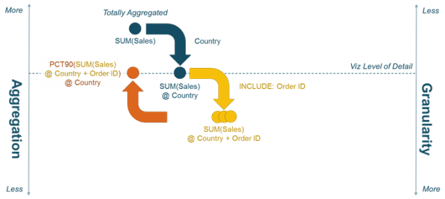
Note that we use the INCLUDE expression so that Orders that are split across Countries are allocated correctly and not double-counted. Some readers might prefer to solve this problem with a FIXED expression, in which case we would need to write:
[Total Sales including Order]
{INCLUDE [Country], [Order ID] : SUM([Sales])}
This would be correct for the required chart but would limit our flexibility to change the grouping to some other dimension (e.g. by Region or by Shipping Type).
3. Table Calculation vs. Level of Detail Expression
This is the decision that many people find confusing. However, the process to choose between a table calculation and an LOD Expression is the same as for a table calculation vs. a basic calculation. You need to ask:
Consider the following example in which we ask: What is the 90th percentile of sales at the order total level, shown by country?
You will notice that this is almost identical to the question asked in #1 above. The only difference is that the percentile calculation is performed on the order total, not the order detail. You may realise the chart on the left side is in fact the same chart as we saw on the right side in #2. We already know the granularity of this problem is different to the data source and the viz, so we should use an LOD Expression.
The chart on the right side is the same as the right chart from #1. However, the dots represent Orders, not Order Details. This is simply done by changing the granularity of the viz (swap Row ID with Order ID on the Detail shelf). Because table calculations keep the calculation logic separate from the computation scope and direction, we don’t even need to change the calculation; just compute using Order ID.
It can get tricky to be sure about the answer to our decision-process questions, and sometimes you can solve a problem one way until you later introduce a complication. Consider the following example where we ask: For each age group, what percent of illnesses does each disease account for?
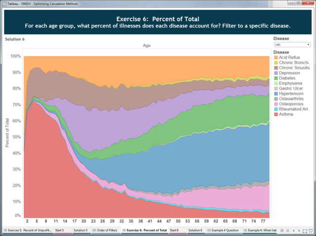
This is clearly a percent-of-total problem and we can very quickly solve this problem with a quick table calculation over the Disease. However, when we then add the complication of allowing the user to filter to a specific disease, we find the following:
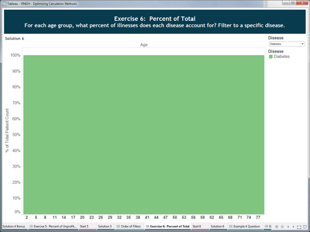
This is because our result set no longer contains all the data we need; the filter has removed the Patient Count data for the other diseases. You could solve this by making the filter a table calculation:
[Filter Disease]
LOOKUP(MIN([Disease]), 0) compute using Disease
Or you can use LOD Expressions, knowing that FIXED calculations are done before dimension filters. First, work out the total number of people in an age group:
[Total Patients per Disease]
{FIXED [Age]:SUM([Patient Count])}
Then you can compute the % total:
[Pct Total]
SUM([Patient Count])/SUM([Total Patients per Disease])
4. When Only Table Calculations Will Do
Finally, we need to add one final concept to our decision process. There are several categories of problems that can only be solved using table calculations:
- Ranking
- Recursion (e.g. cumulative totals)
- Moving calculations (e.g. rolling averages)
- Inter-row calculations (e.g. period vs. period calculations)
So the question to ask here is: Does my problem require the use of ranking, recursion, moving calculations, or inter-row calculations?
This is because table calculations can output multiple values for each partition of data while basic and LOD Expressions output a single value for each partition/grouping of data. Consider the following exercise in which we ask: In the last year, how many times has a stock broken its record close value to date?
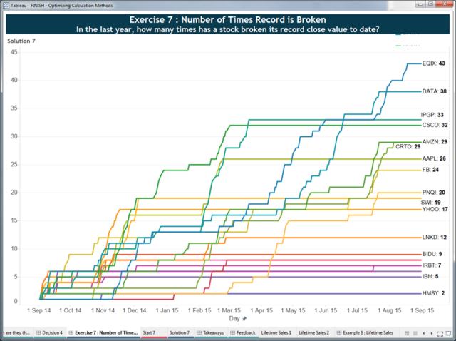
We need a recursive calculation here. I need to consider all the previous values before me in order to tell if I've reached a new maximum. We can do this with a RUNNING_MAX function. So we first calculate the highest value to date:
[Record to Date]
RUNNING_MAX(AVG([Close])) compute using Day
Then at the day level, we need to flag those days where the record was broken:
[Count Days Record Broken]
IF AVG([Close]) = [Record to Date] THEN 1 ELSE 0 END
Finally, we need to count these days:
[Total Times Record Broken]
RUNNING_SUM([Count Days Record Broken]) compute using Day
Lessons Learned
The key takeaways from all this are:
- There is no silver bullet. The answer is always “it depends…” but the decision process will get you started selecting the right approach.
- The layout of the viz matters. And as it changes, you might need to change your calculation type.
- There are scenarios where different solutions perform differently—depending on the volume and complexity of your data, the complexity of the question, and the required layout.
- There are always tradeoffs to consider (performance vs. flexibility, vs. simplicity). A good rule of thumb is that you can pick any two.
For more information and examples, you can download the above workbook here.