Understanding Level of Detail (LOD) Expressions
See how to use and leverage LOD Expressions in your analysis.
At Tableau, our goal is to make data analysis a delightful experience. People tell us that when they are deeply engaged in Tableau they stop thinking about the mechanics of using the product and just have fun asking questions of their data. We call this experience flow—a state of joyful immersion in a task.
If you have to start thinking about how to use the tool to solve the problem, the state of flow is broken. One common cause of this is the need to work with data that has been aggregated to different levels of detail. These questions are often simple to ask, but hard to answer. They often sound something like: Can I plot the number of days per quarter where my company had more than 100 orders?
To address these types of questions, Tableau 9.0 introduces a new syntax called Level of Detail (LOD) Expressions. This new syntax both simplifies and extends Tableau’s calculation language by making it possible to address level of detail questions directly.
In this whitepaper, you’ll gain insights into how LOD Expressions work, along with a more in-depth look at the different types of LOD Expressions and their respective use cases.
At Tableau, our goal is to make data analysis a delightful experience. People tell us that when they are deeply engaged in Tableau they stop thinking about the mechanics of using the product and just have fun asking questions of their data. We call this experience flow—a state of joyful immersion in a task.
If you have to start thinking about how to use the tool to solve the problem, the state of flow is broken. One common cause of this is the need to work with data that has been aggregated to different levels of detail. These questions are often simple to ask, but hard to answer. They often sound something like:
- Can I plot the number of days per quarter where my company had more than 100 orders?
- Find the biggest deal each sales person has ever closed, then show the averages by manager?
- Tag every customer by the year he/she first became a customer, then use that tag to group sales?
To address these types of questions, Tableau 9.0 introduces a new syntax called Level of Detail (LOD) Expressions. This new syntax both simplifies and extends Tableau’s calculation language by making it possible to address level of detail questions directly.
LOD Expressions represent an elegant and powerful way to answer questions involving multiple levels of granularity in a single visualization.
How LOD Expressions Work—Explaining The “Level Of Detail”
A key aspect of exploring data is understanding the structure of the source. For example, you may have restaurant inspection data that at the most granular level is listed by its street address. You may then want to aggregate the data to view properties by zip code, city, state, or even country.
In Tableau, you typically do this by dropping the dimensions you care about into your view (e.g., city, state). Depending on the dimensions you’ve chosen to add to the view, your data will be aggregated accordingly —to the “viz level of detail”, or Viz LOD for short.
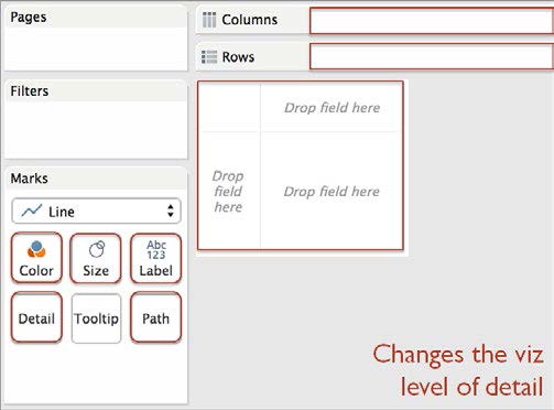
Placing dimensions on the shelves highlighted here will add them to the viz LOD.
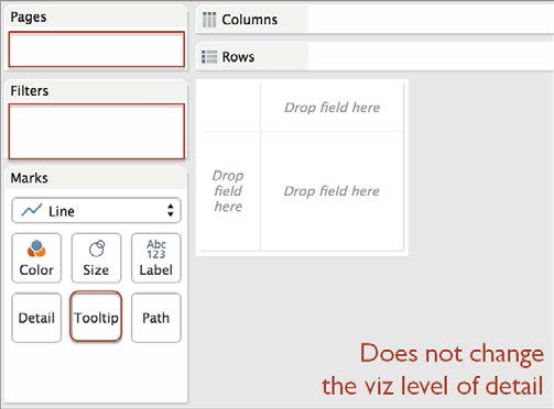
Placing dimensions on the pages, filters and tooltips shelves does not add them to the Viz LOD. Dimensions placed on these shelves are ways of modifying the data in the view without displaying it visually.
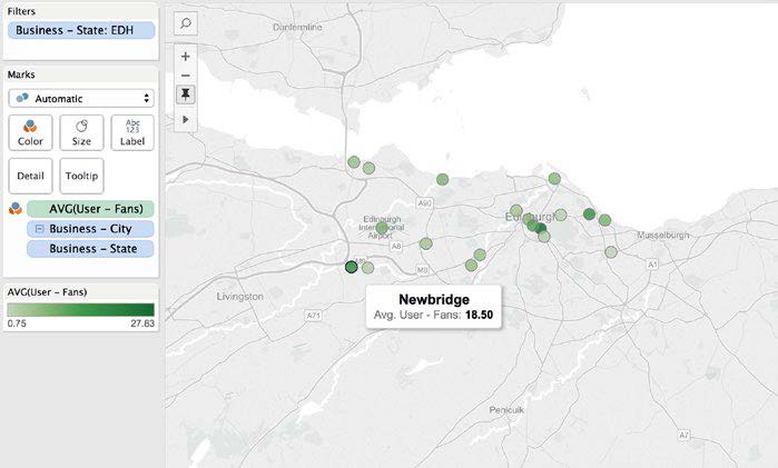
This map shows restaurant inspection data from YELP in the greater Edinburgh area. The data has been aggregated to the City/State level of detail.
The data has been aggregated to the City/State level of detail. The data in the view is aggregated based on the Viz LOD—which in this case consist of City and State— and is more aggregated than the underlying data source. The selected point in the image shows the average user fans for all restaurants in Newbridge, Edinburgh.
Adding more granular dimensions to the view will result in a less aggregated Viz LOD. For instance, we could add Business ID to the visualization (by dropping it on the Detail Shelf), to see the average user fans for every individual business. Doing so will also change the visualization: every single business will appear as a circle on the map. But what if we don’t want the visualization to change? What if we want to determine the total user fans for each Business ID, average those values for each city, and show only one circle per city? What we want to see is the average number of fans per restaurant in each city.
This will require adding an additional dimension to the view without dragging that dimension into the visualization. An LOD expression will allow us to this.
Let’s create a new calculated field called Fans per Business. Here is a brief introduction to the syntax:
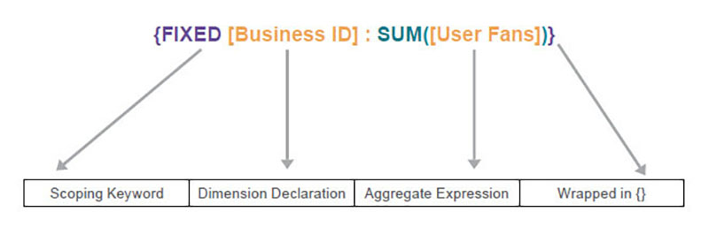
The expression tells Tableau to perform the aggregation for each Business ID, regardless of other dimensions used in the viz. You can use the LOD Expression to calculate the total User Fans per Business ID. After dragging this new field into the view, we can then average those values per city.
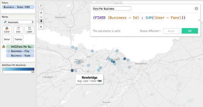
The Fans per Business field has been added to the Color Shelf. Newbridge has the highest average fans per business with 185 fans—a value that was computed using a FIXED LOD expression.
By using the FIXED operator in our LOD Expression, we gain insight into which cities have, on average, more fans per Business ID. Meaning, those cities with a darker shade of blue have more popular restaurants (or the city could have more residents and hence, more total fans per restaurant).
There are three types of LOD expression keywords—EXCLUDE, INCLUDE and FIXED—each of which alters the scope of the LOD expression.
Include: Calculating At A Lower Level Of Detail
In this example, we’ll look at a standard sales database (the Superstore database that comes with Tableau). Here, each row represents the sale of a certain item. Order may contain multiple items and spread across multiple rows. In other words, the deepest level of detail in this database is a unique item.
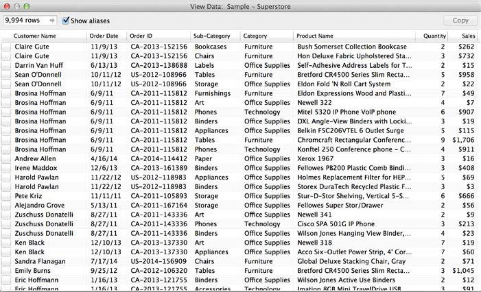
A snapshot of the Superstore database that comes with Tableau.
The first row in this snapshot of the database is for a purchase of 2 Bush Somerset Bookcases. The second row is a purchase of 3 Hon Stacking Chairs. These two rows together comprise a single order—namely, order CA-2013-152156.
Suppose you are analyzing the sales performance of each region and would like to know which region has the highest (or lowest) average order size?
To figure this out, you need to calculate the size of each order (sum the sales corresponding to each Order ID), and then average those values by region.
This business question is easy enough to ask, and with the new LOD Expressions syntax, Tableau makes it easy to answer. Here is a more detailed discussion of the new syntax:
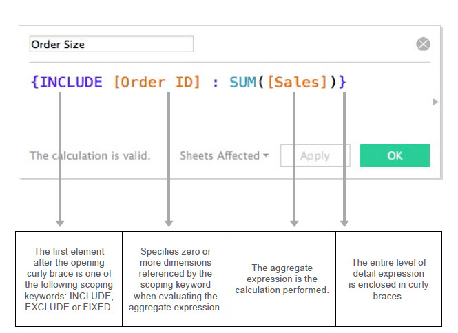
LOD Expressions can be written in the calculation editor as shown here. This LOD expression is
used to sum the purchases in each Order ID. The result is a new field called Order Size.
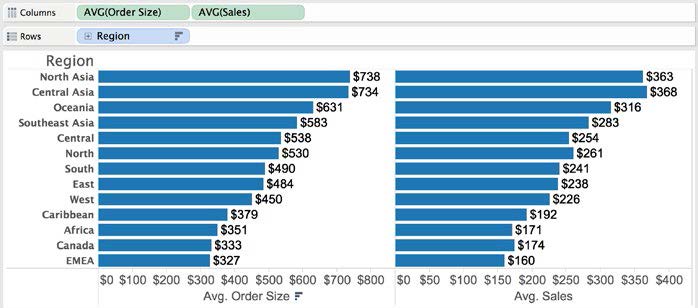
The bars on the left show the average size of orders by Region—computed using an LOD
Expression—while the bars on the right show the average Sales by Region (i.e., the average of
all order line items, regardless of which order they were in). You may now answer the question:
Which Region has the highest average order size?
You can see that North Asia and Central Asia have the highest average Order Size, $737 and $733 respectively. We were able to determine this even though Order ID does not appear in the visualization. (Before Tableau Version 9, we could not have computed these values unless Order ID had been added to the view).
If we had simply plotted Region versus AVG(Sales)—as seen in the bars on the right in the figure— we would see the average of all line items (rows) in each Region, which is not the result we are looking for. In contrast, with the LOD expression Order Size, we are able to first determine the size of each order(i.e. the sum of sales for all line items within that order), and then average the resulting orders by Region to determine average Order Size by Region.
Now that we have a sense of our largest average order size, let’s ask a slightly more complex question: Which country in the sales database has sales reps who close the “biggest deals,” on average? What we want to do is:
- Find the biggest deal (the max deal) that each sales person has ever closed, and then
- Average those ‘biggest deals’ by country.
This question is multi-faceted, but it is easy to answer with an LOD expression:
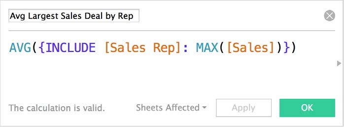
The LOD expression Avg Largest Sales Deal by Rep is used to calculate the average maximum deal per sales rep. In this case, the average of the LOD Expression is typed directly in the calculation editor window.
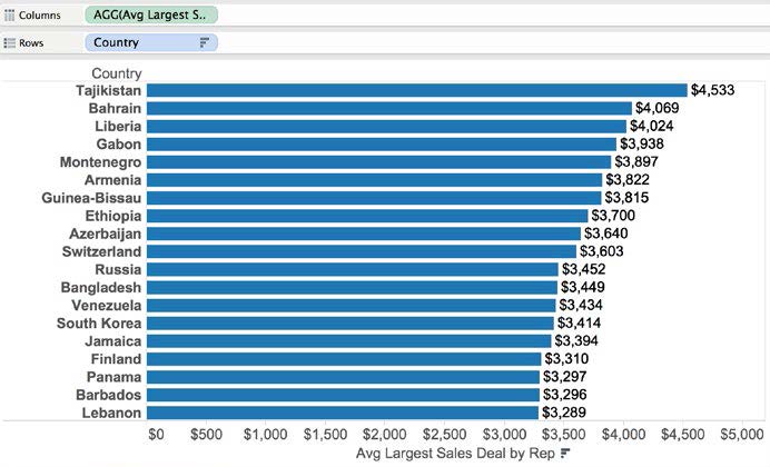
The LOD Expression Avg Largest Sales Deal by Rep allows us to compare the average max deal across Countries. The average “biggest deal” for all sales reps in Tajikistan is $4,533.
Notice that we answered this question with one expression AVG({INCLUDE [Sales Rep] : MAX([Sales])})—no need for complex formulas. In fact, you can ask additional questions of your data by adding additional dimensions to the view, and the calculation will update. For instance, let’s add Year to the analysis:
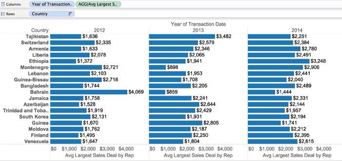
The LOD expression Avg Largest Sales Deal by Rep will update when additional dimensions are added to the view—in this case Year of Transaction Date. The visualization now shows the average “biggest deal” each sales rep closed, by country and year. The average of the “biggest deals” for all sales reps in Tajikistan was $1,636 in 2012, $3,482 in 2013, and $2,251 in 2014.
Using the INCLUDE keyword in the calculation, the Sales Rep field is being explicitly included in the calculation, but so are any other dimensions that are placed in the visualization (in this case Country and Year). By adding Year to the view, we can dive deeper into our analysis and can now gain insights such as this: Bahrain had the largest average “biggest deal” in 2012 with $4,069.
A graphical representation of how Tableau performs an INCLUDE LOD Expression is depicted in the following flow diagram.
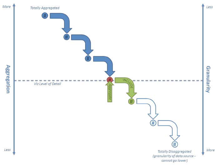
An INCLUDE LOD expression will add the dimension(s) to the viz LOD
The INCLUDE keyword creates an expression that is less aggregated (i.e., more granular) than the Viz LOD. The specified dimension(s) are first added to the viz LOD before calculations are performed.
Notice the INCLUDE Expression is used in the view as an aggregated measure. In fact, all INCLUDE expressions are either used as measures or aggregated measures when placed on the view.
Exclude: Calculating At A Higher Level Of Detail
Consider the following scenario: For each month, we want to see the total Sales, as well as the total sales by Region. To do this:
- We need to exclude Region from our calculation of the monthly Total Sales
- And then include Region when calculating the regional Sales breakdowns.
Let’s explore an additional example using the sales database— as described earlier.
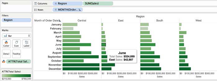
Monthly total Sales (color on bars) is computed using an EXCLUDE LOD expression. The sum of Sales by Region (the length of bars) is not based on an LOD expression. The result is a single visualization showing numbers at two different levels of detail.

This LOD expression, called Total Sales, allows you to compute the monthly total sales across all Regions.
Notice that in the viz above, Region has been placed on the Column shelf and thus contributes to the Viz LOD of Region, Month(Order Date). Using the EXCLUDE expression, you have the ability to calculate the total sales (across all regions) while displaying the regional sales breakdowns. As such, we have created an LOD expression that is “above” the Viz LOD (i.e. less granular): {EXCLUDE [Region] : SUM([Sales])}
A key to the EXCLUDE keyword: Tableau first removes the excluded dimension from the Viz LOD and performs the calculation as if the dimension was not present at all. The result is then displayed visually. A graphical representation of how Tableau performs an EXCLUDE LOD Expression is depicted in the following flow diagram.

Using an EXCLUDE LOD expression will exclude the desired dimension(s) from the calculation.
The expression {EXCLUDE [Region] : SUM([Sales])} tells Tableau to calculate the sum of sales using whatever dimensions are in use in the viz, excluding the Region dimension. This means we end up with a single value for each month which represents the total sales across all regions.
Now we have a powerful view that shows us both total Sales and Sales by Region—both of which use the SUM aggregation.
We can also mix aggregations. For instance, let’s change our LOD Expression to show the average Sales per month, while still showing regional sums:
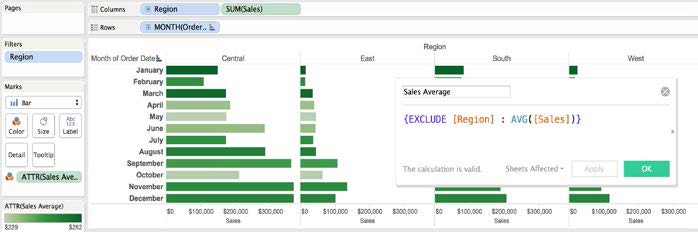
The color now represents the average monthly Sales and is computed using an EXCLUDE LOD expression. The sum of Sales by Region (the length of the bar) is not based on an LOD expression.
Similar to an INCLUDE Expression, all EXCLUDE Expressions are either used as measures or aggregated measures when placed on the view. These types of expressions are great for “percent of total” or “difference from overall average” calculations.
Fixed: Specifying The Exact Level Of Detail
LOD Expressions also open the door to creating an aggregation level completely independent of the Viz LOD; something that was previously only possible by using custom SQL.
As an example, consider the following scenario: Let’s say you’d like to analyze YELP data to find the yearly cohorts in which a business had its first review. Does each cohort have the same review trends?
With LOD Expressions, we can specify the cohort at an exact level of detail:

This LOD expression will fix the level of detail to each Business ID. Then, for each Business ID, it takes all reviews and finds the minimum Year of the Review Date and associates that value with the Business ID. You can imagine First Review Year to be a new column in the database.
When we use this field in the viz, the calculation scope is implicitly defined in the expression. Once the First Review Year is recorded for each Business ID (as shown below), exploring the cohorts can be insightful.

The level of detail has been fixed at Business – ID. Notice the first review year (as found in the FIXED LOD Expression) is the same for each review row.

This visualization shows the Number of Records (number of reviews) broken down by First Review Year and the Year of Review Date. By adding First Review Year to Color, we have created a cohort analysis.
Now, let’s use First Review Year as a filter:
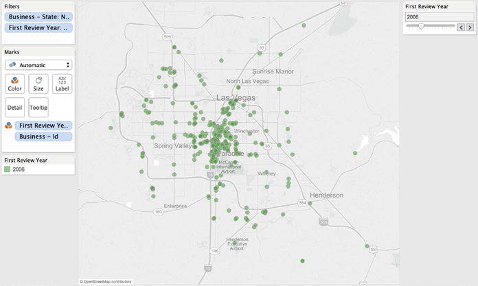
An LOD expression can also be used as a filter. By using a Quick Filter on First Review Year, you can quickly step through the yearly cohorts to see if certain areas of Las Vegas were
first reviewed earlier or later than others. The FIXED LOD Expression is calculated above the Dimension filter on Business – State in the view.
Notice that each yearly cohort has been given a discrete “bin”—that is, First Review Year is used in the view as a dimension. FIXED expressions can be used as dimensions or measures. Depending on the data type, Tableau will place the resulting calculation either as a dimension or a measure.
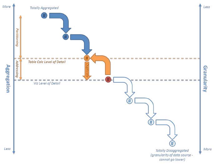
A key distinction between INCLUDE/EXCLUDE and FIXED is where each falls in the filtering hierarchy as shown below. FIXED LOD Expressions are computed before dimension filters and after context filters. This can enable many use cases
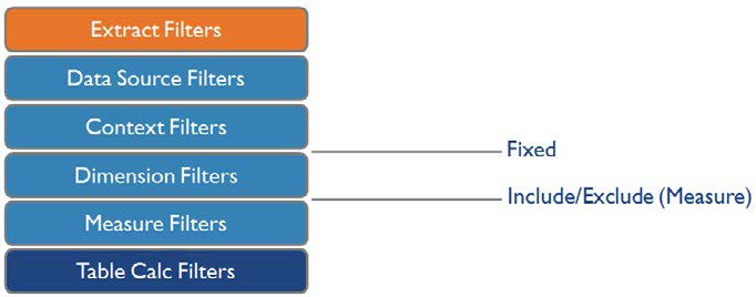
FIXED LOD expression filters are applied after context filters and before dimension filters. On the other hand, INCLUDE/EXCLUDE filters are applied after dimension filters and before measure filters.
Canonical Use Cases
A few useful scenarios for LOD Expressions have been outlined in previous sections of this paper—however, these are only the beginning of the power of using an LOD Expression to solve a business question. Other notable examples:
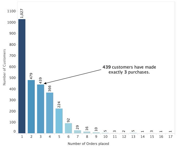
Histogram of Number of Orders: How many customers in each segment have made 1, 2, 3 etc. orders?

For a thorough discussion of some of the best use cases for LOD Expressions, please refer to the Tableau publication “Top 15 LOD Expressions”, which includes online sample workbooks with step-by-step instructions.
Final Thoughts
LOD Expressions are a powerful new capability of Tableau 9.0 that allow us to easily solve problems that previously required complicated formulas. They allow us to intuitively define the scope of calculations and stay in a state of flow as we explore our data.
LOD Expressions are not a new form of Table Calculations; they can replace many Table Calculations, but also open new possibilities. LOD Expressions and Table Calculations operate differently. A Table Calculation is generated exclusively from the result of a query, while an LOD Expression is usually generated as part of the query to the underlying data. Table Calculations always produce measures as their result, while LOD Expressions can create measures, aggregated measures or dimensions.
LOD expressions represent a vital step towards the goal of complete flow, where all questions are simple and elegant to answer.
Appendix A – Additional Resources
For additional resources on creating, using, and explaining LOD Expressions, please refer to the materials listed below.
- First Look: An introduction to LOD Expressions from Robin Cottiss
- Explanation: Level of Detail Expressions from Bora Beran
- Example and Tutorial: Top 15 LOD Expressions
- Example: Craig Bloodworth of the Information Lab records his experience using LOD expressions
Appendix B – LOD Expressions vs. Table Calculations
For people who used Tableau before Version 9, LOD Expressions will allow you to replace calculations you may have authored in more cumbersome ways:
- Using Table Calcs, you may have tried to find the first or last period within a partition. For example, calculating the headcount of an organization on the first day of every month.
- Using Table Calcs, Calculated Fields, and Reference Lines, you may have tried to bin aggregate fields. For example, finding the average of a distinct count of customers.
- Using Data Blending, you may have tried to achieve relative date filtering relative to the maximum date in the data. For example, if your data is refreshed on a weekly basis, computing the year to date totals according to the maximum date.
This appendix is designed for people who first learned Tableau using Version 8 or an earlier release. In those versions of the software, Table Calculations were sometimes used to specify the level of aggregation. Although LOD Expressions now make it easy to pinpoint the level of detail, Table Calcs have not lost their important place in your analysis.
The table below outlines a few key distinctions between Table Calcs and LOD Expressions.

When attempting to achieve the equivalent of an EXCLUDE statement— as seen earlier—a table calc may be difficult to use in a non-convoluted way. You’d need to address all dimensions in the viz as either partitioning or addressing—according to the desired level of detail.
Additionally, because table calculations are aggregated from the query results they can only work “up” from the viz LOD (i.e. more aggregated/less granular).
Using table calculations as a method of specifying the level of detail relies on the table calc level of detail (i.e. setting dimensions as partitioning or addressing).
The addressing fields are the dimensions that you’d like to exclude in the calculation.
On the other hand, if you’d like to achieve the equivalent of an INCLUDE statement using table calcs, you need to make the query results less aggregated to match the lowest level calculation.
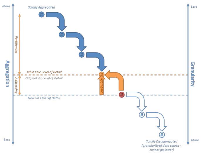
To achieve the same result as an INCLUDE LOD expression prior to Tableau 9.0, you could utilize a table calc to create a new viz LOD.
The next step would be to use table calculations to aggregate back up to the original viz LOD. However there will be more viz LOD records than we need so it’s generally necessary to keep only one using a filter like INDEX()=1 or an equivalent.
As you can see, using a table calc to achieve an EXCLUDE/INCLUDE expression technically arrives at the answer, but could be performed much easier (and quicker) with an LOD expression.