Marey-Inspired PATH Train Schedule

The idea for this visualization has been bouncing around my head for a while now, but I have had a tough time figuring out how to execute it.  The original Marey Train Schedule visualization catalogs trips from Paris to Lyon in 1885.  This visualization may look familiar to you if you're an Edward Tufte fan, as it is on the cover of his book The Visual Display of Quantitative Information.

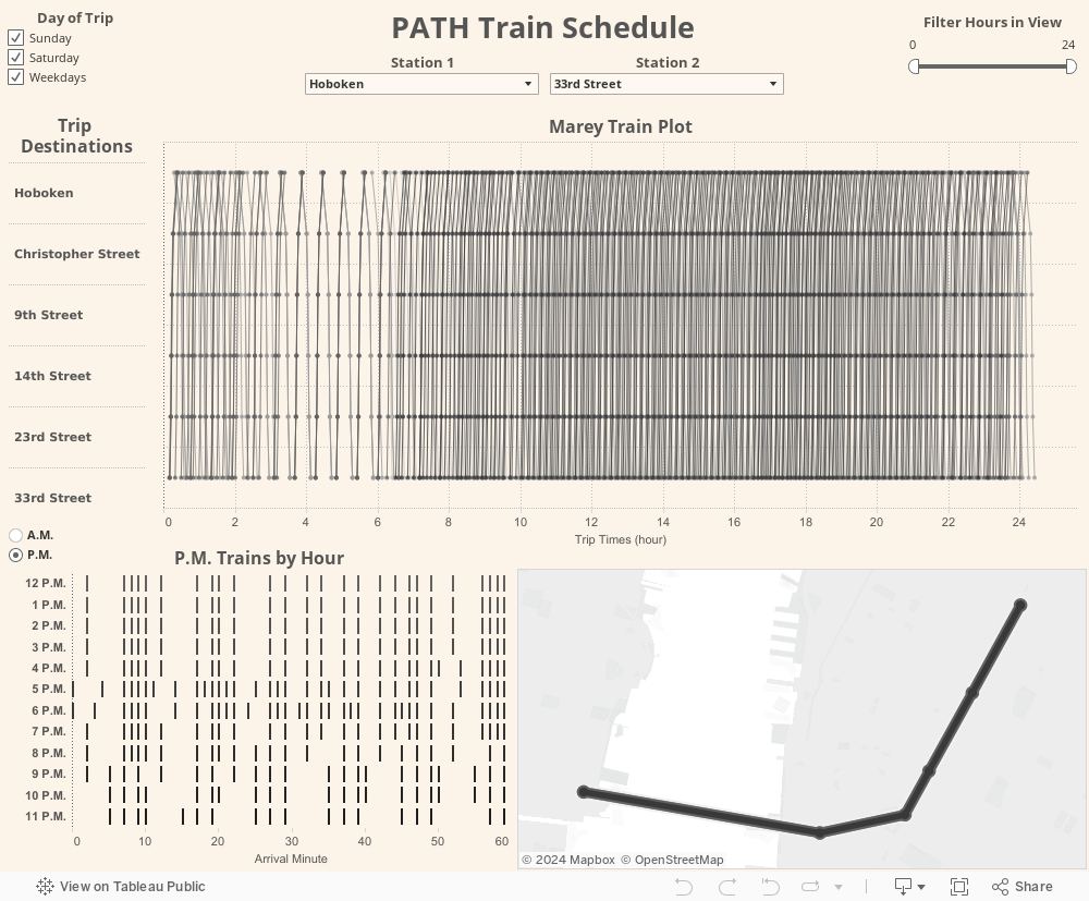
Similar graphs have been created using other technologies in the past (most notably in D3 by Mike Bostock) but I was unable to find anything similar in Tableau.  This visualization focuses on the PATH train that is primarily used to take commuters between New Jersey and New York City.

Use the drop-downs at the top of the page to select a start and end station.  The Marey plot makes up the top half of the page, with some supporting charts for train times and locations below it.

Since this took a bit to figure out, I thought it might be helpful to talk about how I got from the original data source to the end product.  Below the visualization, I have step-by-step instructions detailing the process that led to the end product.  I have also open sourced all of my code on GitHub which you can access here.  If you have any questions, as always, I am happy to answer them on Twitter - @McGovey.

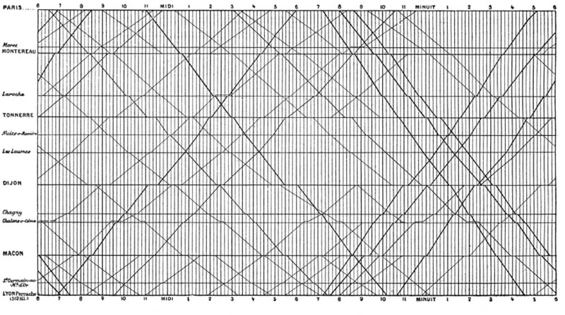
Here is an image of the original.

The only data source was the GTFS formatted PATH data that was pulled into Alteryx, and visualized using Tableau.  To start you can download the full PATH train schedule (or a different GTFS train schedule of your choice).

I knew the Marey Train plot was not something I was going to be able to build in the native data source format so some level of data cleansing was going to be required.  I decided to pull everything into Alteryx and build my tables there.  Below are the specifics of what I had to do in Alteryx for those of you who can't open the yxmd file and see for yourselves.

First, we want a single table to work with as a base, so start by combining the files for routes, individual train trips, station stops, stop times, and days that the train runs.  To build the x-axis for the chart, we need a numeric field; while the arrival_time field in the stop_times table is really helpful, we want to convert that to a decimal format.  For example, 15:30:00 becomes 15.5 (note: the tick marks on the x-axis only use integers).  That's all that is necessary for a single table file but when you try to pull this into Tableau, you have a tough time creating a dynamic station stop parameter.

The stops at each station on a given route will vary based on the time of day and the route taken so if you try to use the stop_sequence, you will get multiple data points per stop.  To get around this, we have to do some work.  For a while, my visualization relied on a field that was built by grouping the data by the route and getting the average time it takes to reach each stop.  This was working fine with an earlier dataset and it wasn't until my Slalom colleague, Pankil Shah, and I switched to the PATH data that we noticed just how big of an issue this approach would cause.  So instead, what we're going to try to ultimately achieve is a unique list of the possible origins and destinations paired with the possible stops between them.

We do this by creating a cross tab (column-wise format) of all the possible stations for a given train trip, then joining it back to the original table on trip ID.  This gives us data in this format:

trip_id	station	arrtime	station1name	station2name
1	station1name	0.2	0.2	0.3
2	station2name	0.3	0.2	0.3
3	station3name	0.6		0.3
4	station4name	0.1	0.5

Once this table has been created, transpose this back into a vertical format and filter out the values where there aren't values for both the origin and destination stations, to get a list of possible stations.  To match all unique destination-origin pairs, a TransitID value is created from the above list.

The unique destination-origin pair list is then joined to the original table on trip ID which will create a giant list of all possible stops for a given trip.  To get to a more manageable data set, filter out any stations that do not occur between the time of departure and the time of arrival.

Finally, to get the y-axis, calculate the average time it takes to get to each stop between the selected origin destination pair. Start by filtering for only trains going in one direction (not return trips, otherwise our averages would be miscalculated) then finding the minimum station time for each trip (or you can think of it as the trip start time).  Next you need to find the time that it takes to reach each station on a trip.  Once you have these two points, subtract the trip start time from the station stop time.  Then average the result of that to get the average time it takes to get to each station.  I know that's a lot so I posted an image of a close up of that process in Alteryx.

Quick side note: an earlier version of this Tableau viz used level of detail calculations. I didn't realize just how powerful these calculations are and how much you can achieve using them.

I have already talked about how I created the sequence order and the arrival time number but I also included trip_id detail for each of the lines, route_id and direction_id for the colors, and added sequence order to the path shelf (otherwise there would be gaps in the lines for stations that were skipped).  The only thing left to do is create the station filters.

To start, I created a station 1 and station 2 parameter.  These will drive the stations that you're viewing.  These parameters control the visualization via a calculated field (used as a filter) that checks if the name of station 1 is equal to the origin name and station 2 is equal to the destination name.  There is also an OR clause included to make sure you can view trains going in both directions.

And that's all there is to it.

I hope you were able to follow along and that you will be able to use some of the stuff in here to create some cool visualizations on your own. If I lost you at any point, I highly recommend taking a look at the files and digging into some of the details to determine what exactly is going on.  I know this may have seemed rather technical but I'm really happy that I was able to get a working version of a historically significant chart.